52. Two-Dimensional Test of Unsaturated-Saturated Transport
This example first appeared as scenario 6 in (Morway et al., 2013). At that time, new capabilities programmed into MT3DMS (Zheng & Wang, 1999) allowed for simulation of solute transport in the unsaturated-zone using flux terms calculated by the unsaturated-zone flow (UZF1; (Niswonger et al., 2006)) package. (Morway et al., 2013) referred to the published MT3DMS variant as UZF-MT3DMS. Eventually, however, these capabilities were better documented and released with MT3D-USGS (Bedekar et al., 2016). For the purpose of testing unsaturated-zone transport using the UZF/UZT packages inside MODFLOW 6, the MODFLOW 6 solution is compared against the MT3D-USGS solution. Moreover, we note that the results of the MT3D-USGS simulation were compared to results calculated by VS2DT (Lappala et al., 1987) for establishing the accuracy of the MT3D solution. VS2DT solves Richards’ equation and as such can simulate flow and solute fluxes across the unsaturated-saturated interface. Therefore, this example problem tests the ability of MODFLOW 6 to accurately simulate the infiltration, unsaturated-zone transport, recharge, and subsequent saturated transport of dissolved solute.
Currently, the UZT package inside MODFLOW 6 does not simulate dispersion in the unsaturated zone. As a result, two scenarios were setup in both MT3D-USGS and MODFLOW 6. The first maintains fidelity with (Morway et al., 2013) and simulates dispersion in the unsaturate zone. In the second scenario, no dispersion is simulated in the unsaturated zone by setting the longitudinal, transverse, and vertical dispersion equal to zero in the upper 11 layers as summarized in the following table. Brackets (“[ ]”) in the table indicate a list of values, one per layer, is used to define the value for the entire layer. Where only one value appears inside the brackets, a constant value is used throughout the model domain.
Scenario |
Scenario Name |
Parameter |
Value |
|---|---|---|---|
1 |
e x-gwt-uzt-2d-a |
longitudina l dispersivity (\(m\)) |
[0.5] |
rat io horizontal to longitudina l dispersivity (unitless) |
[0.4] |
||
r atio vertical to longitudina l dispersivity (unknown) |
[0.4] |
||
2 |
e x-gwt-uzt-2d-b |
longitudina l dispersivity (\(m\)) |
[0.0, 0.0, 0.0, 0.0, 0.0, 0.0, 0.0, 0.0, 0.0, 0.0, 0.0, 0.0, 0.5, 0.5, 0.5, 0.5, 0.5, 0.5, 0.5, 0.5] |
rat io horizontal to longitudina l dispersivity (unitless) |
[0.0, 0.0, 0.0, 0.0, 0.0, 0.0, 0.0, 0.0, 0.0, 0.0, 0.0, 0.0, 0.0, 0.4, 0.4, 0.4, 0.4, 0.4, 0.4, 0.4, 0.4] |
||
r atio vertical to longitudina l dispersivity (unknown) |
[0.0, 0.0, 0.0, 0.0, 0.0, 0.0, 0.0, 0.0, 0.0, 0.0, 0.0, 0.0, 0.0, 0.4, 0.4, 0.4, 0.4, 0.4, 0.4, 0.4, 0.4] |
52.1. Example description
For this problem, a relatively small, two-dimensional profile that is 10 \(m\) wide by 5 \(m\) deep is used. Layer thickness, as well as the column widths, are 0.25 \(m\). A constant head boundary of 1.625 \(m\) is set on the left and right sides of the active model domain. An infiltration rate of 0.1 \(m/day\) is specified all along the top boundary except for the left- and right-most columns where the constant head boundary condition exists. A no-flow boundary is used along the bottom of the simulation domain. The simulation domain starts out clean; however, solute enters with the infiltrating water in the middle 10 columns only. Additional model parameter values are listed in Table 52.2.
Parameter |
Value |
|---|---|
Number of layers |
20 |
Number of rows |
1 |
Number of columns |
40 |
Column width (\(m\)) |
0.25 |
Row width (\(m\)) |
0.25 |
Layer thickness (\(m\)) |
0.25 |
Top of the model (\(m\)) |
5.0 |
Horizontal hydraulic conductivity (\(m/day\)) |
2.5 |
Vertical hydraulic conductivity (\(m/day\)) |
0.5 |
Aquifer storativity |
1e-5 |
Specific yield |
0.35 |
Residual water content |
0.1 |
Saturated water content |
0.45 |
Initial water content |
0.105 |
Brooks-Corey Epsilon |
4.0 |
Infiltration rate (\(m/d\)) |
0.1 |
Concentration of recharge in select cells(\(ppm\)) |
1.0 |
Porosity |
0.45 |
Longitudinal dispersivity (\(ft\)) |
0.5 |
Ratio of horizontal transverse dispersivity to longitudinal dispersivity |
0.4 |
Ratio of vertical transverse dispersivity to longitudinal dispersivity |
0.4 |
Simulation time (\(days\)) |
60.0 |
Given the relatively dry initial condition within the unsaturated zone, the infiltrating front reaches the water table on day 8 of the 60 day simulation period. Once the infiltrating wave reaches the saturated zone, the water table rises into the unsaturated zone and further tests the accuracy of the transport solution.
52.2. Example results
Because MODFLOW 6 does not (yet) simulate dispersion in the unsaturated-zone, there are some significant differences between the two solutions (Figure 52.1). Whereas longitudinal and transverse dispersive fluxes spread solute ahead and to the side of the downward migrating plume within the MT3D-USGS unsaturated zone solution, the UZF/UZT formulation within MODFLOW 6 simulates purely advective transport in the unsaturated zone. However, once solute reaches the saturated zone, dispersion is simulated using the XT3D package (the default setting).
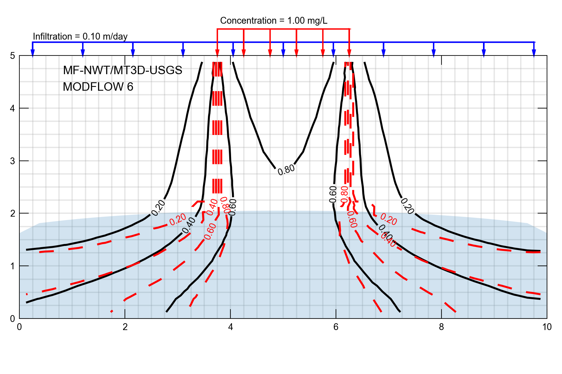
Figure 52.1 A two-dimensional problem first published in (Morway et al., 2013). MT3D-USGS results closely match a benchmark solution calculated by VS2DT (Lappala et al., 1987). The light blue shaded region shows the location of the saturated zone.
A second scenario in which longitudinal, transverse, and vertical dispersion are set equal to zero in the unsaturated zone of the MT3D-USGS solution was run. Because this setup more closely mimics the MODFLOW 6 unsaturated zone solution, results between the respective models more closely match one another. We note, however, that because many transport problems originate at land surface, the final transport solution within the satured zone may ultimately depend on accurately simulating unsaturated zone transport processes. That is, the extent and severity of the saturated zone plume may be inextricably tied to the spread and delay of migrating solute in the unsaturated zone, as demonstrated by the two different solutions within the saturated zone when dispersion is and is not accounted for in the unsaturated zone.
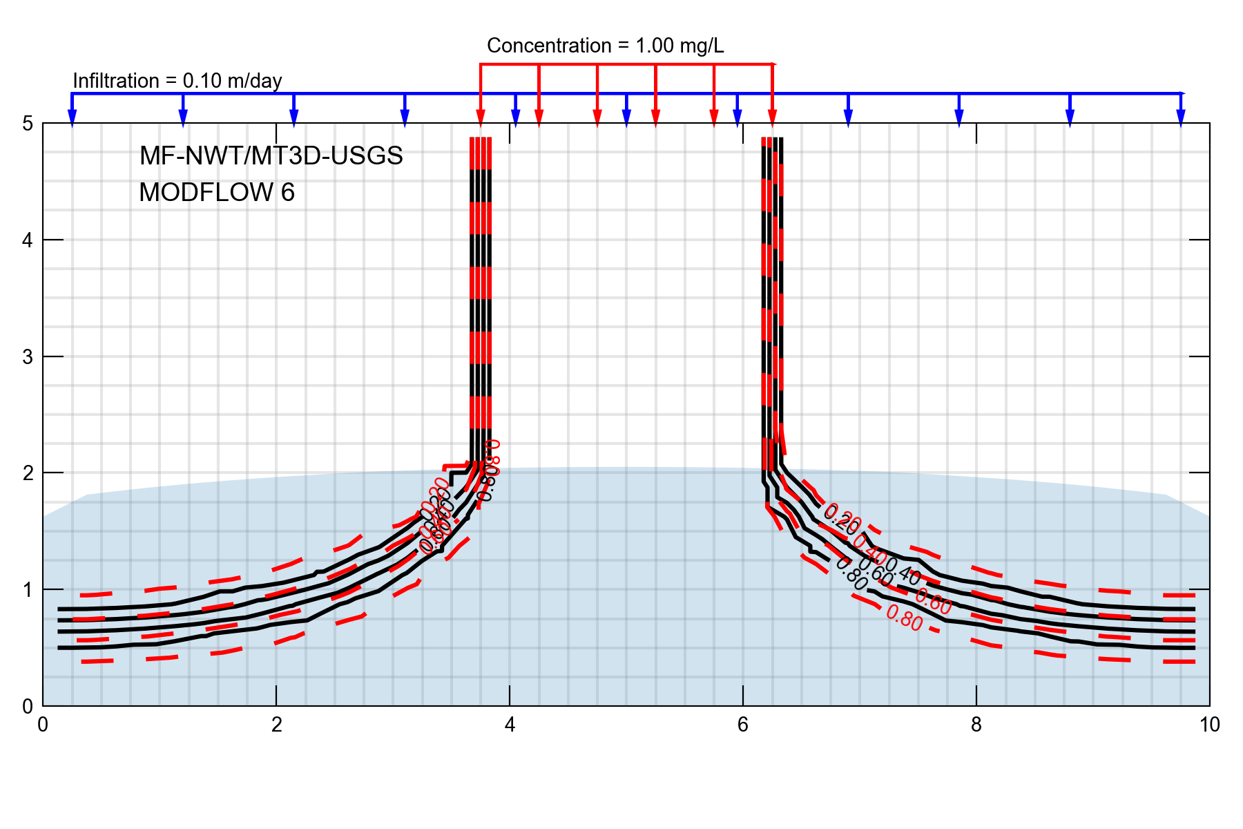
Figure 52.2 A two-dimensional transport problem with no dispersive fluxes in either MODFLOW 6 or MT3D-USGS within the unsaturated-zone. The light blue shaded region shows the location of the saturated zone.
52.3. References Cited
Bedekar, V., Morway, E. D., Langevin, C. D., & Tonkin, M. J. (2016). MT3D-USGS version 1: A U.S. Geological Survey release of MT3DMS updated with new and expanded transport capabilities for use with MODFLOW. https://doi.org/10.3133/tm6a53
Lappala, E. G., Healy, R. W., Weeks, E. P., & others. (1987). Documentation of computer program VS2D to solve the equations of fluid flow in variably saturated porous media. Retrieved from https://pubs.er.usgs.gov/publication/wri834099
Morway, E. D., Niswonger, R. G., Langevin, C. D., Bailey, R. T., & Healy, R. W. (2013). Modeling variably saturated subsurface solute transport with MODFLOW-UZF and MT3DMS. Groundwater, 51(2), 237–251. https://doi.org/10.1111/j.1745-6584.2012.00971.x
Niswonger, R. G., Prudic, D. E., & Regan, R. S. (2006). Documentation of the Unsaturated-Zone Flow (UZF1) package for modeling unsaturated flow between the land surface and the water table with MODFLOW-2005. Retrieved from https://pubs.usgs.gov/tm/2006/tm6a19/
Zheng, C., & Wang, P. P. (1999). MT3DMS—a modular three-dimensional multi-species transport model for simulation of advection, dispersion and chemical reactions of contaminants in groundwater systems; documentation and user’s guide.
52.4. Jupyter Notebook
The Jupyter notebook used to create the MODFLOW 6 input files for this example and post-process the results is: