31. Sagehen UZF1 Package Problem 1
The first test problem in (Niswonger et al., 2006) presents a conceptual model of the Sagehen watershed that showcased the first version of the unsaturated-zone flow (UZF1) package. The Sagehen watershed is located on the eastern side of the northern Sierra Nevada, north of Lake Tahoe and the city of Truckee (see inset in Figure 31.1). The simulation spans the upper 27 \(mi^2\) of the watershed. The lowest land surface altitude of 1,928 \(m\) above mean sea level occurs where Sagehen Creek exits the model. The highest altitude of 2,649 \(m\) above mean sea level occurs on the western-most crest of the watershed, resulting in roughly 720 \(m\) of topographic relief across the watershed. Figure 31.1 depicts the setting and topographic relief of the watershed. The geologic setting is primarily comprised of volcanic rocks overlain with a veneer of alluvium. Annual precipitation averages approximately 970 \(mm\) which falls primarily in the form of snow.
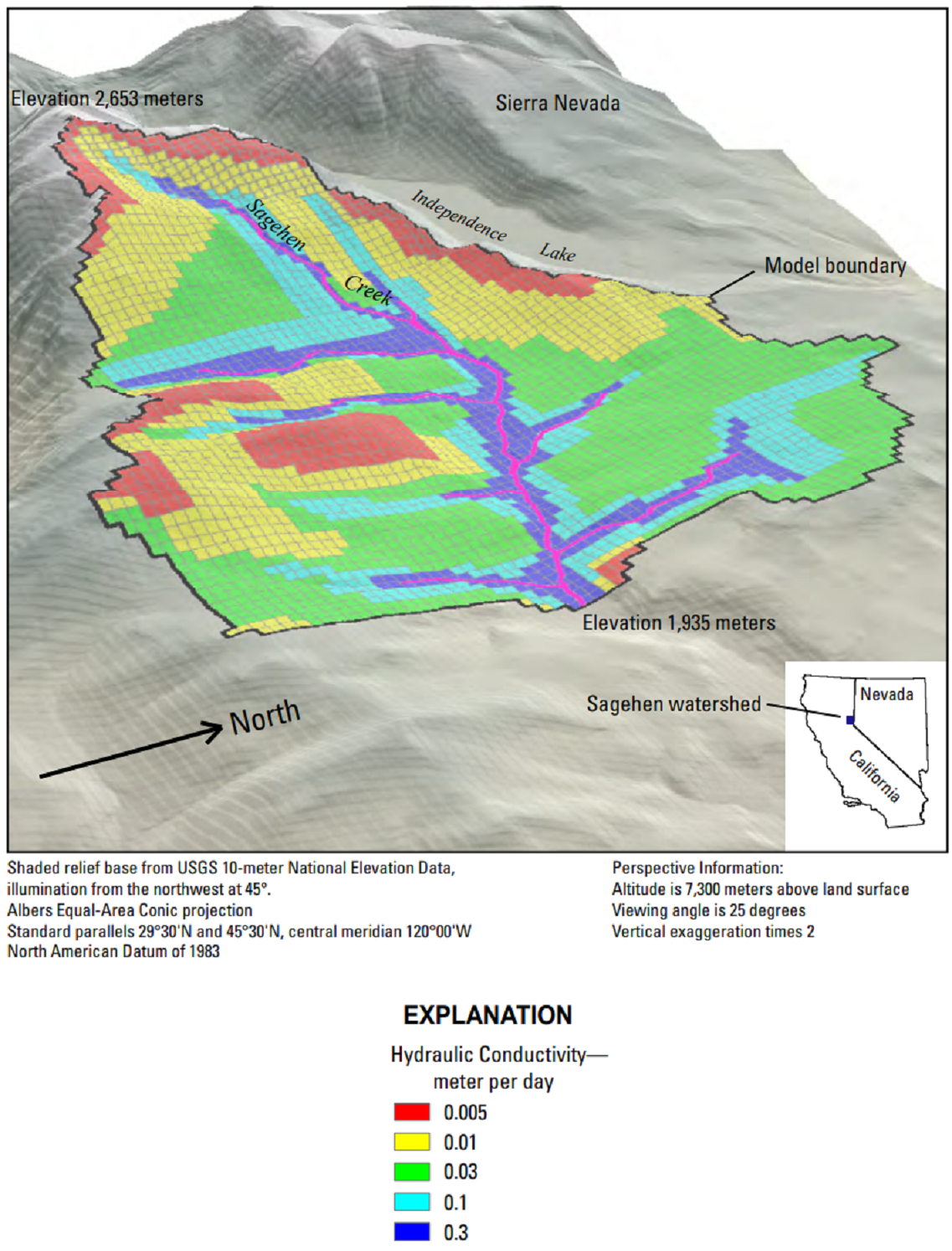
Figure 31.1 3-Dimensional perspective view of the Sagehen watershed looking westward. Colors depict zones of varying hydraulic conductivity within the active grid domain.
31.1. Example description
For this MODFLOW 6 demonstration of the Sagehen model, a single model layer ranging between 53 \(m\) and 899 \(m\) thick is used to represent both the saturated and unsaturated zones. Spatially, 73 rows and 81 columns with uniform 90 \(\times\) 90 \(m\) grid cells are used to represent the watershed. The simulated period uses daily stress periods with one time-step per stress period, starting on December 1st and ending on November 30th. The first stress period is steady state, while all others are transient. Because the perimeter of the active model domain follows a topographic watershed divide, a no-flow boundary is used around the perimeter and bottom of the groundwater flow model. However, the cell hosting Sagehen Creek at its exit point as well as the two adjacent cells were specified constant head cells. The specified vertical hydraulic conductivity of the unsaturated zone was set equal to the vertical hydraulic conductivity used in the node-property flow (NPF) package. The stream network is represented with 213 inter-connected stream reaches, all with a constant width of 3 \(m\) and range from 30 to 114 \(m\) in length.
A set of infiltration factors shown in Figure 31.2 tie precipitation rates to land-surface altitude to account for the orographically-driven variations in precipitation. Infiltration factors are three times greater along the western crest of the watershed compared to the lower valley elevations near the outlet. The infiltration factors were multiplied by infiltration rates that varied daily as shown by the “infiltration” time series shown in Figure 31.4.
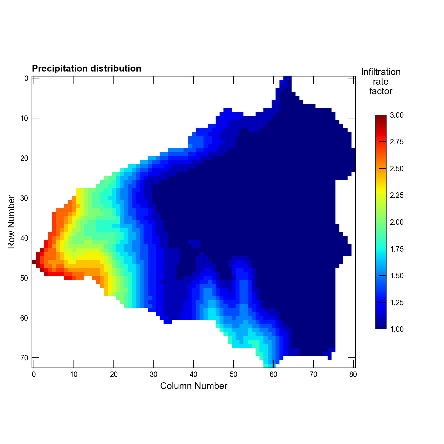
Figure 31.2 Plot of static infiltration factors used to spatially vary infiltration rates within the watershed. Infiltration factors were multiplied by a time series of infiltration rates shown in Figure 31.4
The water content in the unsaturated zone is calculated based on the flux through, and properties of, the unsaturated-zone during the initial steady-state stress period when the recharge rate equals the specified infiltration rate at land surface. A uniform extinction depth of 2.5 \(m\) is applied across the entire model. Below 2.5 \(m\), Evapotranspiration (ET) ceases. Using the same approach implemented in UZF1 (Niswonger et al., 2006), water is first removed from the unsaturated zone in fulfillment of the ET demand. Any remaining residual ET demand is then satisfied using water in the saturated zone when the water table is within 2.5 \(m\) of land surface. An extinction water content of 0.10 was specified for the entire model
A summary of model parameter values are listed in Table 31.1. Interested readers are referred to (Niswonger et al., 2006) for a discussion of additional details, including how the distribution of hydraulic conductivity was derived and aspects of the model calibration, among others.
Parameter |
Value |
|---|---|
Number of layers in parent model |
1 |
Number of rows in parent model |
73 |
Number of columns in parent model |
81 |
Parent model column width (\(m\)) |
90.0 |
Parent model row width (\(m\)) |
90.0 |
Horizontal hydraulic conductivity (\(m/d\)) |
0.005 – 0.3 |
Vertical hydraulic conductivity (\(m/d\)) |
0.01 – 0.3 |
Specific Yield |
0.1 – 0.2 |
Saturated water content |
0.15 – 0.25 |
Extinction water content |
0.10 |
Saturated hydraulic conductivity of unsaturated zone |
0.005 – 0.3 |
Brooks-Corey Epsilon |
4.0 |
Number of SFR stream reaches |
213 |
Hydraulic conductivity of streambed (\(m/d\)) |
0.3 |
Width of stream reaches (\(m\)) |
3 |
Streambed thickness (\(m\)) |
1 |
31.2. Example results
Figure 31.3 shows the calculated depth to groundwater during the steady-state stress period. Depths to groundwater varied significantly over the model domain, ranging from more than 25 \(m\) below land surface to at, or slightly above, land surface near streams.
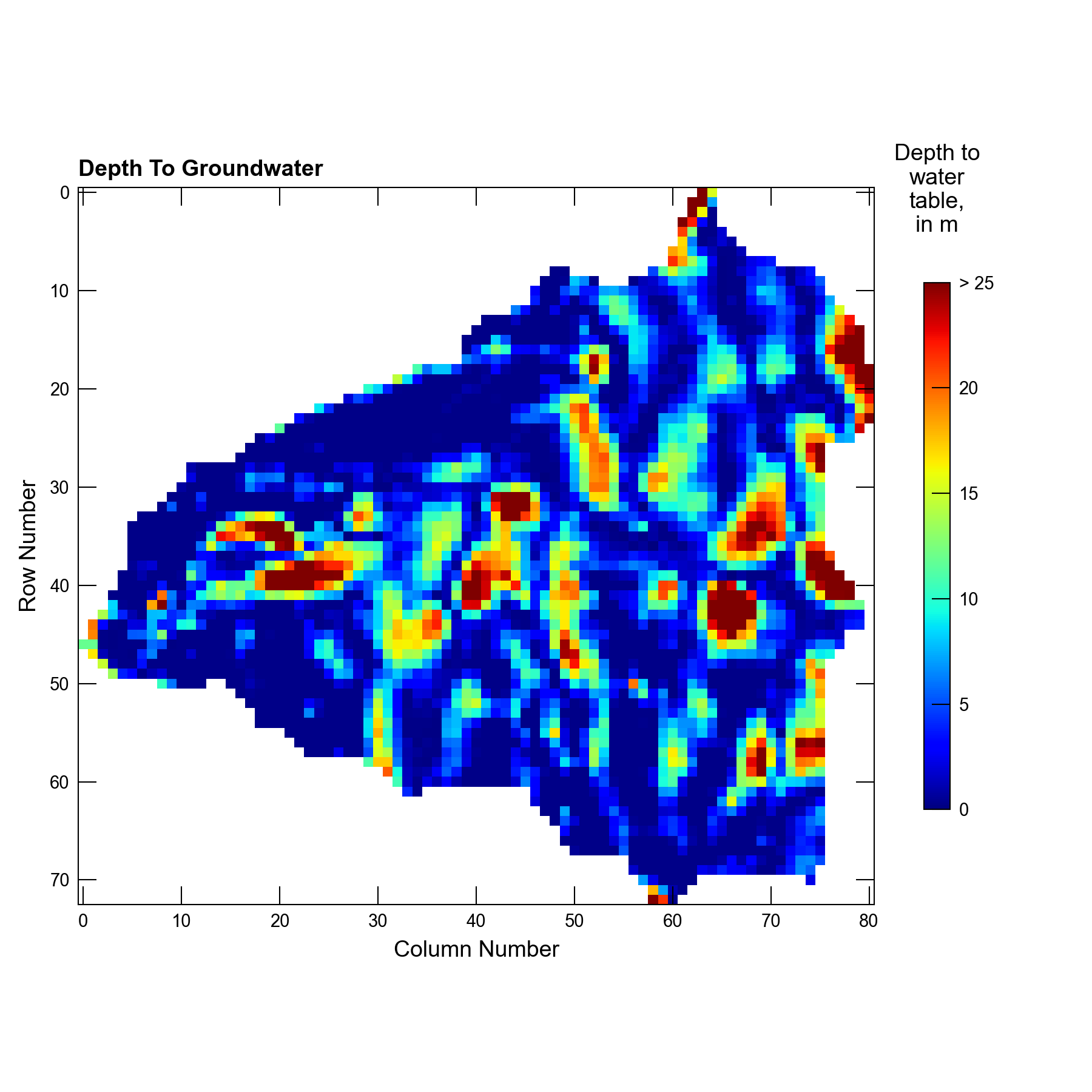
Figure 31.3 Calculated depth to groundwater during the steady-state stress period at the beginning of the simulation.
The UZF2 package partitions infiltration into runoff, resulting from saturation excess and/or rejected infiltration; recharge; ET; and changes in unsatruated zone storage (Langevin et al., 2017). Although changes in unsaturated zone storage are not shown, Figure 31.4 shows how the infiltration was partitioned among recharge and ET through time. Runoff processes are depicted in Figure 31.5, and together with groundwater discharge directly to streams equal the total streamflow generated by the watershed.
A noteworthy enhancement between this version of the model and that first documented in (Niswonger et al., 2006) is that the drain (DRN) package has been added to the model to capture groundwater discharge to land-surface. In this way, groundwater discharge is kept separate from rejected infiltration, enabling easier viewing of the relative contribution of each of these processes since they are now separated in the calculated model budget. The UZF2 package could be used to simulate both processes; however, if this approach is used the relative contribution of groundwater discharge to land surface and rejected infiltration to stream flow are lumped. In flow-only simulations, this approach may suffice. In a groundwater transport simulation, where these two contributing sources to stream flow may have very different concentrations, the approach taken here will enable improved tracking of solute contributions to surface water. In addition to the DRN package, the mover (MVR) package has been invoked to deliver groundwater discharge and rejected infiltration to the nearest downgradient (i.e., downhill) stream reach. Previously, the IRUNBND array in UZF1 was used to route groundwater discharge and rejected infiltration to the stream network.
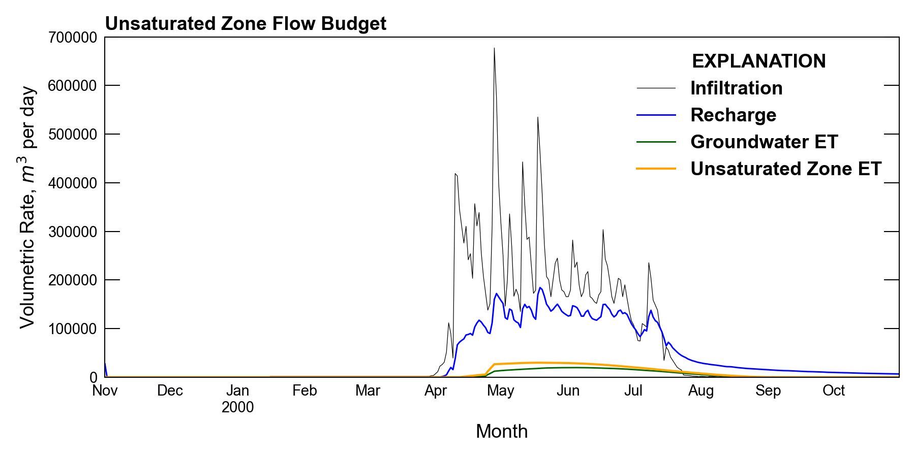
Figure 31.4 Volumetric rates of infiltration, recharge, and evapotranspiration from the unsaturated and saturated zones summed over the model domain.
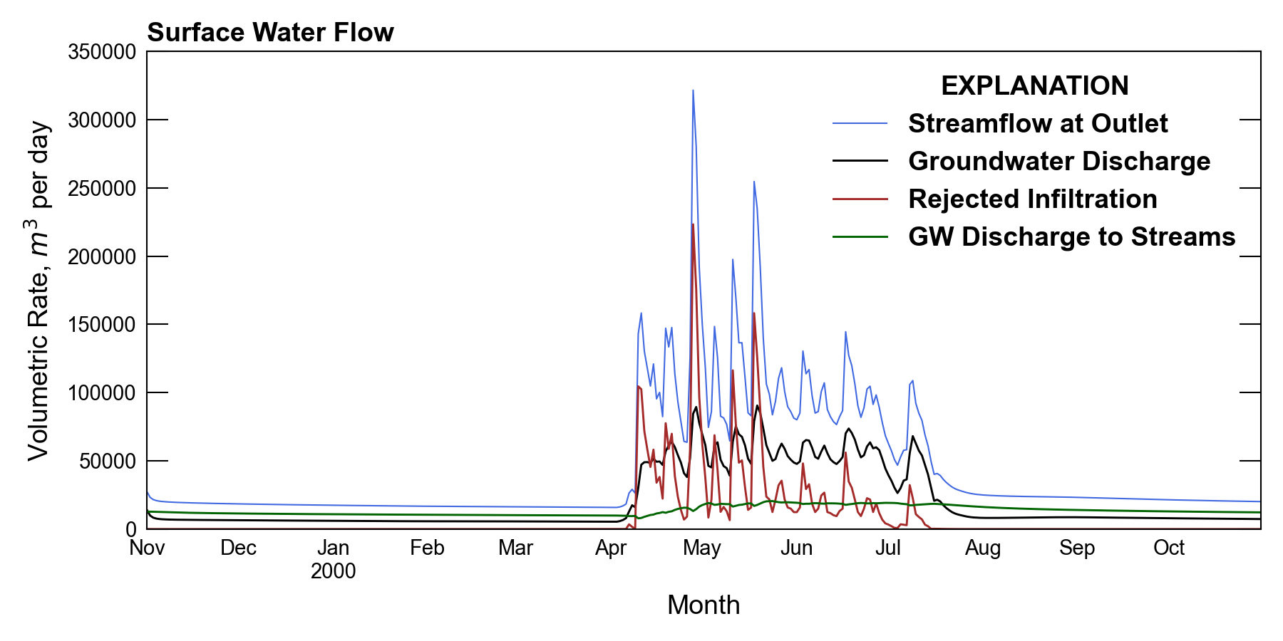
Figure 31.5 Volumetric flow rates of surface-water generation and runoff.
31.3. References Cited
Langevin, C. D., Hughes, J. D., Provost, A. M., Banta, E. R., Niswonger, R. G., & Panday, S. (2017). MODFLOW 6, the U.S. Geological Survey Modular Hydrologic Model. https://doi.org/10.5066/F76Q1VQV
Niswonger, R. G., Prudic, D. E., & Regan, R. S. (2006). Documentation of the Unsaturated-Zone Flow (UZF1) package for modeling unsaturated flow between the land surface and the water table with MODFLOW-2005. Retrieved from https://pubs.usgs.gov/tm/2006/tm6a19/
31.4. Jupyter Notebook
The Jupyter notebook used to create the MODFLOW 6 input files for this example and post-process the results is: