16. Neville-Tonkin Multi-Aquifer Well Problem
This is the multi-aquifer well simulation described in (Neville & Tonkin, 2004). The example simulates an upper and lower aquifer separated by an impermeable confining unit but connected by a well that is open across both aquifers.
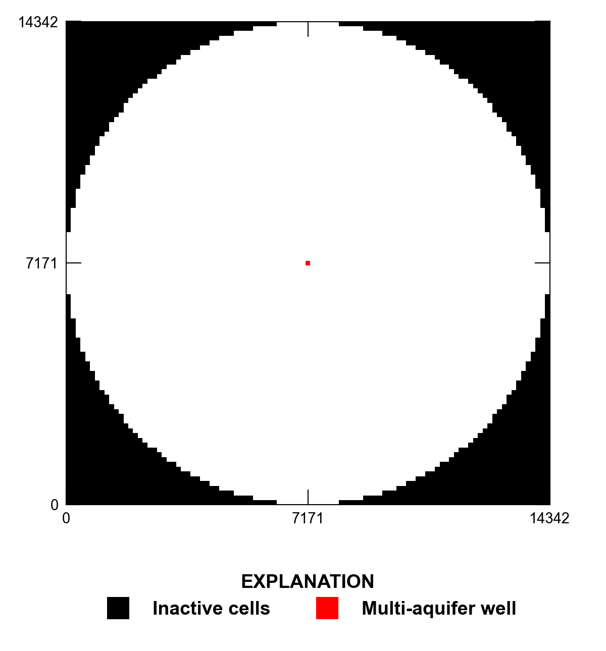
Figure 16.1 Location of inactive cells and the multi-aquifer well.
16.1. Example Description
Model parameters for the example are summarized in
Table 16.1. The model consists of a grid of
101 columns, 101 rows, and 2 layers. The model domain is 14,342
\(m\) in the x- and y-directions
(Figure 16.1). The discretization is in the
row and column directions is 142 \(m\). The top of the model is
specified to be -50 \(m\) and the bottom of each layer is specified
to be 142.9 and -514.5 \(m\). Groundwater flow was inactivated
beyond a distance of 7,163 \(m\) from the center cell (row 51,
column 51) in model layers 1 and 2 by specifying an IDOMAIN value of
zero in these cells (Figure 16.1).
One transient stress period 2.1314815 days in length is simulated. The stress period has 50 time steps and uses a time step multiplier equal to 1.2, which results in time step lengths that range \(0.51 \times 10^{-4}\) to \(0.39\) days. A short simulation time is specified to prevent the effect of the well propagating to the model boundary.
Parameter |
Value |
|---|---|
Number of periods |
1 |
Number of layers |
2 |
Number of rows |
101 |
Number of columns |
101 |
Column width (\(m\)) |
142.0 |
Row width (\(m\)) |
142.0 |
Top of the model (\(m\)) |
–50.0 |
Bottom elevations (\(m\)) |
–142.9, –514.5 |
Starting head (\(m\)) |
3.05, 9.14 |
Horizontal hydraulic conductivity (\(m/d\)) |
1.0 |
Vertical hydraulic conductivity (\(m/d\)) |
1.0e-16 |
Specific storage (\(1/d\)) |
1e-4 |
Well radius (\(m\)) |
0.15 |
The horizontal and vertical hydraulic conductivity is 1 and \(1 \times 10^{-16}\) \(m/d\). The transmissivity of of the upper and lower aquifer is 92.9 and 371.6 \(m^2/d\). A constant specific storage value of \(1 \times 10^{-4}\) (\(1/d\)) is specified. All model layers are specified to be confined. An initial head of 3.05 and 9.14 \(m\) are specified in the upper and lower aquifer, respectively.
The multi-aquifer well was the only boundary condition specified in the model. The well is located in the center of the model domain (Figure 16.1), fully penetrates both aquifers, and has a well radius of 0.15 \(m\). The Thiem conductance equation was used to calculate the well conductance in each aquifer. The initial head in the well was set equal to the initial head in the lower aquifer (9.14 \(m\)) and well storage was not simulated.
16.2. Example Results
The model was run for the case where the well was not pumping and a case where the well is pumping 1,767 \(m^{3}/d\). Transient results for non-pumping and pumping case are shown in Figure 16.2. For the non-pumping case, the flow from the lower aquifer is balanced by flow to the upper aquifer (Figure 16.2A). The water level in the multi-aquifer well under non-pumping can be calculated using the Sokol solution (Sokol, 1963). The Sokol solution is
where \(h_w\) is the water-level in the well (L), \(T_m\) is the aquifer transmissivity (L\(^{2}\)/T), and \(h_m\) is the aquifer head at the outer-constant head boundary (L). For the non-pumping case, the water-level in the well calculated using equation 16.1 is 7.922 \(m\), which is identical the water-level in the multi-aquifer well.
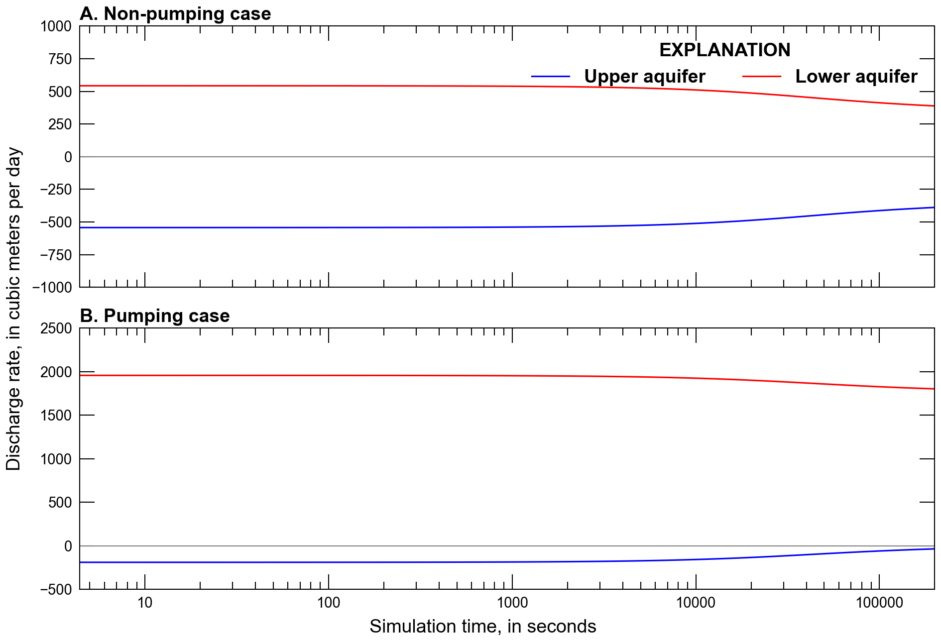
Figure 16.2 Simulated aquifer discharges to the multi-aquifer well. Discharge rates are relative to the multi-aquifer well; positive and negative discharge rates represent inflow to and outflow from the multi-aquifer, respectively. A. Non-pumping case. B. Pumping case.
For the pumping case, the flow from the upper aquifer is actually initially negative, indicating that at early time water flows up the wellbore and into the upper aquifer, rather than discharging from it (Figure 16.2B).
16.3. References Cited
Neville, C. J., & Tonkin, M. J. (2004). Modeling multiaquifer wells with MODFLOW. Ground Water, 42(6), 910–919. https://doi.org/10.1111/j.1745-6584.2004.t01-9-.x
Sokol, D. (1963). Position and fluctuations of water level in wells perforated in more than one aquifer. Journal of Geophysical Research, 68(4), 1079–1080. https://doi.org/10.1029/JZ068i004p01079
16.4. Jupyter Notebook
The Jupyter notebook used to create the MODFLOW 6 input files for this example and post-process the results is: