MOC3D Problem 2 with Triangular Grid
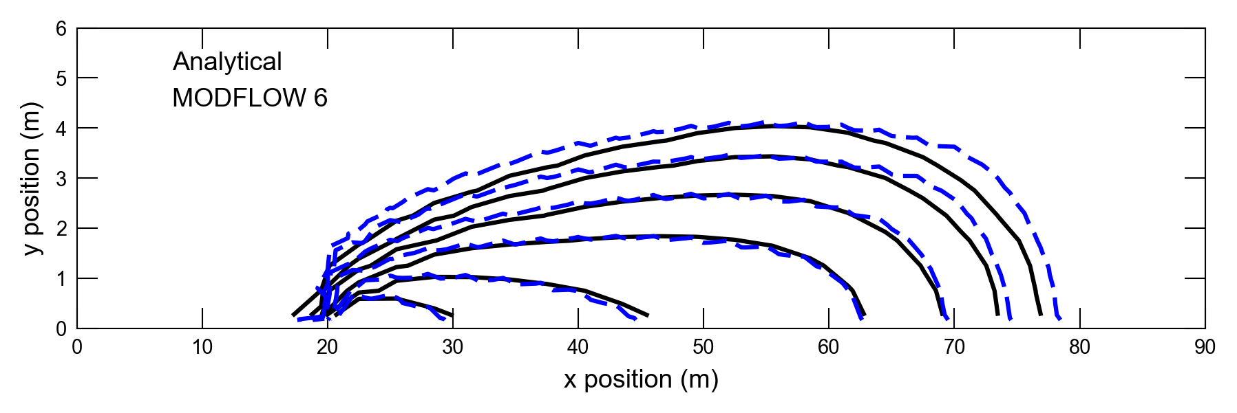
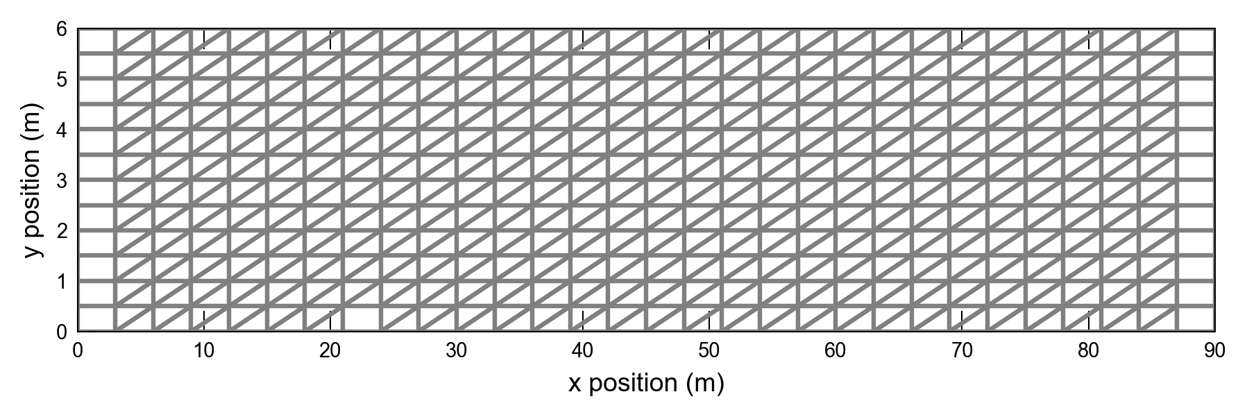
This problem corresponds to the second problem presented in the MOC3D report Konikow 1996, which involves the transport of a dissolved constituent in a steady, three-dimensional flow field. An analytical solution for this problem is given by Wexler 1992. Like the previous example, this example is simulated with a GWT model which receives flow information from a separate simulation with the GWF model. In this example, however, a triangular grid is used for the flow and transport simulation. Results from the GWT model are compared with the results from the Wexler 1992 analytical solution.
Initial setup
Import dependencies, define the example name and workspace, and read settings from environment variables.
[1]:
from pathlib import Path

import flopy
import flopy.utils.cvfdutil
import git
import matplotlib.pyplot as plt
import numpy as np
from flopy.plot.styles import styles
from modflow_devtools.misc import get_env, timed
from scipy.special import erfc

# Example name and workspace paths. If this example is running
# in the git repository, use the folder structure described in
# the README. Otherwise just use the current working directory.
example_name = "ex-gwt-moc3d-p02tg"
try:
    root = Path(git.Repo(".", search_parent_directories=True).working_dir)
except:
    root = None
workspace = root / "examples" if root else Path.cwd()
figs_path = root / "figures" if root else Path.cwd()

# Settings from environment variables
write = get_env("WRITE", True)
run = get_env("RUN", True)
plot = get_env("PLOT", True)
plot_show = get_env("PLOT_SHOW", True)
plot_save = get_env("PLOT_SAVE", True)
Define parameters
Define model units, parameters and other settings.
[2]:
# Model units
length_units = "meters"
time_units = "days"

# Model parameters
nper = 1  # Number of periods
nlay = 40  # Number of layers
nrow = 12  # Number of rows
ncol = 30  # Number of columns
delr = 3  # Column width ($m$)
delc = 0.5  # Row width ($m$)
delv = 0.05  # Layer thickness ($m$)
top = 0.0  # Top of the model ($m$)
bottom = -2.0  # Model bottom elevation ($m$)
velocity_x = 0.1  # Velocity in x-direction ($m d^{-1}$)
hydraulic_conductivity = 0.0125  # Hydraulic conductivity ($m d^{-1}$)
porosity = 0.25  # Porosity of mobile domain (unitless)
alpha_l = 0.6  # Longitudinal dispersivity ($m$)
alpha_th = 0.03  # Transverse horizontal dispersivity ($m$)
alpha_tv = 0.006  # Transverse vertical dispersivity ($m$)
total_time = 400.0  # Simulation time ($d$)
solute_mass_flux = 2.5  # Solute mass flux ($g d^{-1}$)
source_location = (1, 12, 8)  # Source location (layer, row, column)

botm = [-(k + 1) * delv for k in range(nlay)]
specific_discharge = velocity_x * porosity
source_location0 = tuple(idx - 1 for idx in source_location)
Model setup
Define functions to build models, write input files, and run the simulation.
[3]:
class Wexler3d:
    """
    Analytical solution for 3D transport with inflow at a well with a
    specified concentration.
    Wexler Page 47
    """

    def calcgamma(self, x, y, z, xc, yc, zc, dx, dy, dz):
        gam = np.sqrt((x - xc) ** 2 + dx / dy * (y - yc) ** 2 + dx / dz * (z - zc) ** 2)
        return gam

    def calcbeta(self, v, dx, gam, lam):
        beta = np.sqrt(v**2 + 4.0 * dx * gam * lam)
        return beta

    def analytical(self, x, y, z, t, v, xc, yc, zc, dx, dy, dz, n, q, lam=0.0, c0=1.0):
        gam = self.calcgamma(x, y, z, xc, yc, zc, dx, dy, dz)
        beta = self.calcbeta(v, dx, gam, lam)
        term1 = (
            c0
            * q
            * np.exp(v * (x - xc) / 2.0 / dx)
            / 8.0
            / n
            / np.pi
            / gam
            / np.sqrt(dy * dz)
        )
        term2 = np.exp(gam * beta / 2.0 / dx) * erfc(
            (gam + beta * t) / 2.0 / np.sqrt(dx * t)
        )
        term3 = np.exp(-gam * beta / 2.0 / dx) * erfc(
            (gam - beta * t) / 2.0 / np.sqrt(dx * t)
        )
        return term1 * (term2 + term3)

    def multiwell(self, x, y, z, t, v, xc, yc, zc, dx, dy, dz, n, ql, lam=0.0, c0=1.0):
        shape = self.analytical(
            x, y, z, t, v, xc[0], yc[0], zc[0], dx, dy, dz, n, ql[0], lam
        ).shape
        result = np.zeros(shape)
        for xx, yy, zz, q in zip(xc, yc, zc, ql):
            result += self.analytical(
                x, y, z, t, v, xx, yy, zz, dx, dy, dz, n, q, lam, c0
            )
        return result


def grid_triangulator(itri, delr, delc):
    regular_grid = flopy.discretization.StructuredGrid(delc, delr)
    vertdict = {}
    icell = 0
    for i in range(nrow):
        for j in range(ncol):
            vs = regular_grid.get_cell_vertices(i, j)
            vs.reverse()
            if itri[i, j] == 0:
                vertdict[icell] = [vs[0], vs[3], vs[2], vs[1], vs[0]]
                icell += 1
            elif itri[i, j] == 1:
                vertdict[icell] = [vs[0], vs[3], vs[1], vs[0]]
                icell += 1
                vertdict[icell] = [vs[1], vs[3], vs[2], vs[1]]
                icell += 1
            elif itri[i, j] == 2:
                vertdict[icell] = [vs[0], vs[2], vs[1], vs[0]]
                icell += 1
                vertdict[icell] = [vs[0], vs[3], vs[2], vs[0]]
                icell += 1
            else:
                raise Exception(f"Unknown itri value: {itri[i, j]}")
    verts, iverts = flopy.utils.cvfdutil.to_cvfd(vertdict)
    return verts, iverts


def cvfd_to_cell2d(verts, iverts):
    vertices = []
    for i in range(verts.shape[0]):
        x = verts[i, 0]
        y = verts[i, 1]
        vertices.append([i, x, y])
    cell2d = []
    for icell2d, vs in enumerate(iverts):
        points = [tuple(verts[ip]) for ip in vs]
        xc, yc = flopy.utils.cvfdutil.centroid_of_polygon(points)
        cell2d.append([icell2d, xc, yc, len(vs), *vs])
    return vertices, cell2d


def make_grid():
    # itri 0 means do not split the cell
    # itri 1 means split from upper right to lower left
    # itri 2 means split from upper left to lower right
    itri = np.zeros((nrow, ncol), dtype=int)
    itri[:, 1 : ncol - 1] = 2
    itri[source_location0[1], source_location0[2]] = 0
    delra = delr * np.ones(ncol, dtype=float)
    delca = delc * np.ones(nrow, dtype=float)
    verts, iverts = grid_triangulator(itri, delra, delca)
    vertices, cell2d = cvfd_to_cell2d(verts, iverts)

    # A grid array that has the cellnumber of the first triangular cell in
    # the original grid
    itricellnum = np.empty((nrow, ncol), dtype=int)
    icell = 0
    for i in range(nrow):
        for j in range(ncol):
            itricellnum[i, j] = icell
            if itri[i, j] != 0:
                icell += 2
            else:
                icell += 1
    return vertices, cell2d, itricellnum


def build_mf6gwf(sim_folder):
    print(f"Building mf6gwf model...{sim_folder}")
    name = "flow"
    sim_ws = workspace / sim_folder / "mf6gwf"
    sim = flopy.mf6.MFSimulation(sim_name=name, sim_ws=sim_ws, exe_name="mf6")
    tdis_ds = ((total_time, 1, 1.0),)
    flopy.mf6.ModflowTdis(sim, nper=nper, perioddata=tdis_ds, time_units=time_units)
    flopy.mf6.ModflowIms(
        sim,
        print_option="summary",
        inner_maximum=300,
        inner_dvclose=1e-4,
        linear_acceleration="bicgstab",
    )
    gwf = flopy.mf6.ModflowGwf(sim, modelname=name, save_flows=True)
    vertices, cell2d, itricellnum = make_grid()
    flopy.mf6.ModflowGwfdisv(
        gwf,
        length_units=length_units,
        nlay=nlay,
        nvert=len(vertices),
        ncpl=len(cell2d),
        vertices=vertices,
        cell2d=cell2d,
        top=top,
        botm=botm,
    )
    flopy.mf6.ModflowGwfnpf(
        gwf,
        xt3doptions=True,
        save_specific_discharge=True,
        save_saturation=True,
        icelltype=0,
        k=hydraulic_conductivity,
    )
    flopy.mf6.ModflowGwfic(gwf, strt=0.0)
    chdspd = []
    welspd = []
    for k in range(nlay):
        for i in range(nrow):
            icpl = itricellnum[i, ncol - 1]
            rec = [(k, icpl), 0.0]
            chdspd.append(rec)
            icpl = itricellnum[i, 0]
            rec = [(k, icpl), specific_discharge * delc * delv]
            welspd.append(rec)
    flopy.mf6.ModflowGwfchd(gwf, stress_period_data=chdspd)
    flopy.mf6.ModflowGwfwel(gwf, stress_period_data=welspd)
    head_filerecord = f"{name}.hds"
    budget_filerecord = f"{name}.bud"
    flopy.mf6.ModflowGwfoc(
        gwf,
        head_filerecord=head_filerecord,
        budget_filerecord=budget_filerecord,
        saverecord=[("HEAD", "ALL"), ("BUDGET", "ALL")],
    )
    return sim


def build_mf6gwt(sim_folder):
    print(f"Building mf6gwt model...{sim_folder}")
    name = "trans"
    sim_ws = workspace / sim_folder / "mf6gwt"
    sim = flopy.mf6.MFSimulation(sim_name=name, sim_ws=sim_ws, exe_name="mf6")
    tdis_ds = ((total_time, 100, 1.0),)
    flopy.mf6.ModflowTdis(sim, nper=nper, perioddata=tdis_ds, time_units=time_units)
    flopy.mf6.ModflowIms(
        sim,
        print_option="SUMMARY",
        outer_dvclose=0.01,
        inner_dvclose=0.01,
        under_relaxation="simple",
        under_relaxation_gamma=0.9,
        relaxation_factor=0.99,
        linear_acceleration="bicgstab",
    )
    gwt = flopy.mf6.ModflowGwt(sim, modelname=name, save_flows=True)
    vertices, cell2d, itricellnum = make_grid()
    flopy.mf6.ModflowGwfdisv(
        gwt,
        length_units=length_units,
        nlay=nlay,
        nvert=len(vertices),
        ncpl=len(cell2d),
        vertices=vertices,
        cell2d=cell2d,
        top=top,
        botm=botm,
    )
    flopy.mf6.ModflowGwtic(gwt, strt=0)
    flopy.mf6.ModflowGwtmst(gwt, porosity=porosity)
    flopy.mf6.ModflowGwtadv(gwt, scheme="TVD")
    flopy.mf6.ModflowGwtdsp(
        gwt,
        alh=alpha_l,
        ath1=alpha_th,
        ath2=alpha_tv,
    )
    pd = [
        ("GWFHEAD", "../mf6gwf/flow.hds", None),
        ("GWFBUDGET", "../mf6gwf/flow.bud", None),
    ]
    flopy.mf6.ModflowGwtfmi(gwt, packagedata=pd)
    sourcerecarray = [[]]
    icpl = itricellnum[source_location0[1], source_location0[2]]
    srcspd = [[(0, icpl), solute_mass_flux]]
    flopy.mf6.ModflowGwtsrc(gwt, stress_period_data=srcspd)
    flopy.mf6.ModflowGwtssm(gwt, sources=sourcerecarray)
    obs_data = {
        f"{name}.obs.csv": [
            ("SOURCELOC", "CONCENTRATION", source_location0),
        ],
    }
    obs_package = flopy.mf6.ModflowUtlobs(
        gwt, digits=10, print_input=True, continuous=obs_data
    )
    flopy.mf6.ModflowGwtoc(
        gwt,
        budget_filerecord=f"{name}.cbc",
        concentration_filerecord=f"{name}.ucn",
        saverecord=[("CONCENTRATION", "ALL"), ("BUDGET", "LAST")],
        printrecord=[("CONCENTRATION", "LAST"), ("BUDGET", "LAST")],
    )
    return sim


def build_models(sim_name):
    return build_mf6gwf(sim_name), build_mf6gwt(sim_name)


def write_models(sims, silent=True):
    sim_mf6gwf, sim_mf6gwt = sims
    sim_mf6gwf.write_simulation(silent=silent)
    sim_mf6gwt.write_simulation(silent=silent)


@timed
def run_models(sims, silent=True):
    for sim in sims:
        success, buff = sim.run_simulation(silent=silent)
        assert success, buff
Plotting results
Define functions to plot model results.
[4]:
# Figure properties
figure_size = (6, 4)


def plot_analytical(ax, levels):
    n = porosity
    v = velocity_x
    al = alpha_l
    ath = alpha_th
    atv = alpha_tv
    c0 = 10.0
    xc = [22.5]
    yc = [0]
    zc = [0]
    q = [1.0]
    dx = v * al
    dy = v * ath
    dz = v * atv
    lam = 0.0
    x = np.arange(0 + delr / 2.0, ncol * delr + delr / 2.0, delr)
    y = np.arange(0 + delc / 2.0, nrow * delc + delc / 2.0, delc)
    x, y = np.meshgrid(x, y)
    z = 0
    t = 400.0
    c400 = Wexler3d().multiwell(x, y, z, t, v, xc, yc, zc, dx, dy, dz, n, q, lam, c0)
    cs = ax.contour(x, y, c400, levels=levels, colors="k")
    return cs


def plot_grid(sims):
    _, sim_mf6gwt = sims
    with styles.USGSMap():
        sim_ws = Path(sim_mf6gwt.simulation_data.mfpath.get_sim_path())
        fig, axs = plt.subplots(1, 1, figsize=figure_size, dpi=300, tight_layout=True)
        gwt = sim_mf6gwt.trans
        pmv = flopy.plot.PlotMapView(model=gwt, ax=axs)
        pmv.plot_grid()
        axs.set_xlabel("x position (m)")
        axs.set_ylabel("y position (m)")
        axs.set_aspect(4.0)

        if plot_show:
            plt.show()
        if plot_save:
            sim_folder = sim_ws.parent.name
            fname = f"{sim_folder}-grid.png"
            fpth = figs_path / fname
            fig.savefig(fpth)


def plot_results(sims):
    _, sim_mf6gwt = sims
    with styles.USGSMap():
        gwt = sim_mf6gwt.get_model("trans")
        conc = gwt.output.concentration().get_data()

        fig, axs = plt.subplots(1, 1, figsize=figure_size, dpi=300, tight_layout=True)

        gwt = sim_mf6gwt.trans
        pmv = flopy.plot.PlotMapView(model=gwt, ax=axs)
        # pmv.plot_array(conc, alpha=0.5)
        # pmv.plot_grid()
        levels = [1, 3, 10, 30, 100, 300]
        cs1 = plot_analytical(axs, levels)
        cs2 = pmv.contour_array(conc, colors="blue", linestyles="--", levels=levels)
        axs.set_xlabel("x position (m)")
        axs.set_ylabel("y position (m)")
        axs.set_aspect(4.0)

        labels = ["Analytical", "MODFLOW 6"]
        lines = [cs1.collections[0], cs2.collections[0]]
        axs.legend(lines, labels, loc="upper left")

        if plot_show:
            plt.show()
        if plot_save:
            sim_ws = Path(sim_mf6gwt.simulation_data.mfpath.get_sim_path())
            sim_folder = sim_ws.parent.name
            fname = f"{sim_folder}-map.png"
            fpth = figs_path / fname
            fig.savefig(fpth)
Running the example
Define and invoke a function to run the example scenario, then plot results.
[5]:
def scenario(idx, silent=True):
    sims = build_models(example_name)
    if write:
        write_models(sims, silent=silent)
    if run:
        run_models(sims, silent=silent)
    if plot:
        plot_grid(sims)
        plot_results(sims)


scenario(0)
Building mf6gwf model...ex-gwt-moc3d-p02tg
Building mf6gwt model...ex-gwt-moc3d-p02tg
run_models took 19919.05 ms
/tmp/ipykernel_11002/1454031079.py:71: MatplotlibDeprecationWarning: The collections attribute was deprecated in Matplotlib 3.8 and will be removed in 3.10.
  lines = [cs1.collections[0], cs2.collections[0]]
/tmp/ipykernel_11002/1454031079.py:71: MatplotlibDeprecationWarning: The collections attribute was deprecated in Matplotlib 3.8 and will be removed in 3.10.
  lines = [cs1.collections[0], cs2.collections[0]]