This page was generated from
ex-gwf-u1disv.py.
It's also available as a notebook.
Nested Grid Problem
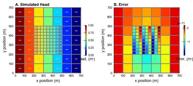
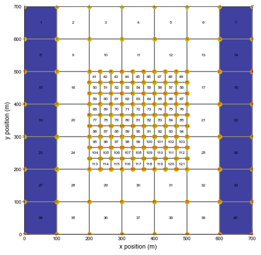
This example shows how the MODFLOW 6 DISV Package can be used to simulate a nested grid problem. The example corresponds to the first example described in the MODFLOW-USG documentation. The problem is run without and with the XT3D option of the NPF Package to improve the solution.
Initial setup
Import dependencies, define the example name and workspace, and read settings from environment variables.
[1]:
from pathlib import Path

import flopy
import flopy.utils.cvfdutil
import git
import matplotlib.pyplot as plt
import numpy as np
from flopy.plot.styles import styles
from flopy.utils.lgrutil import Lgr
from modflow_devtools.misc import get_env, timed

# Example name and workspace paths. If this example is running
# in the git repository, use the folder structure described in
# the README. Otherwise just use the current working directory.
try:
    root = Path(git.Repo(".", search_parent_directories=True).working_dir)
except:
    root = None
workspace = root / "examples" if root else Path.cwd()
figs_path = root / "figures" if root else Path.cwd()

# Settings from environment variables
write = get_env("WRITE", True)
run = get_env("RUN", True)
plot = get_env("PLOT", True)
plot_show = get_env("PLOT_SHOW", True)
plot_save = get_env("PLOT_SAVE", True)
Define parameters
Define model units, parameters and other settings.
[2]:
# Model units
length_units = "meters"
time_units = "days"

# Scenario-specific parameters
parameters = {
    "ex-gwf-u1disv": {
        "xt3d": False,
    },
    "ex-gwf-u1disv-x": {
        "xt3d": True,
    },
}

# Model parameters
nper = 1  # Number of periods
nlay = 1  # Number of layers
top = 0.0  # Top of the model ($m$)
botm = -100.0  # Layer bottom elevations ($m$)
strt = 0.0  # Starting head ($m$)
icelltype = 0  # Cell conversion type
k11 = 1.0  # Horizontal hydraulic conductivity ($m/d$)

# Static temporal data used by TDIS file
# Simulation has 1 steady stress period (1 day)
# and 3 transient stress periods (10 days each).
# Each transient stress period has 120 2-hour time steps.
perlen = [1.0]
nstp = [1]
tsmult = [1.0, 1.0, 1.0]
tdis_ds = list(zip(perlen, nstp, tsmult))

# create the outer grid
nlay = 1
nrow = ncol = 7
delr = 100.0 * np.ones(ncol)
delc = 100.0 * np.ones(nrow)
tp = np.zeros((nrow, ncol))
bt = -100.0 * np.ones((nlay, nrow, ncol))
parent_grid = flopy.discretization.StructuredGrid(delr=delr, delc=delc, top=tp, botm=bt)

# refine the grid and get the disv grid arguments
refine_mask = np.ones((nlay, nrow, ncol))
refine_mask[:, 2:5, 2:5] = 0
lgr = Lgr.from_parent_grid(parent_grid, refine_mask=refine_mask)
grid_props = lgr.to_disv_gridprops()

# Solver parameters
nouter = 50
ninner = 100
hclose = 1e-9
rclose = 1e-6
/home/runner/work/modflow6-examples/modflow6-examples/modflow6-examples/.pixi/envs/default/lib/python3.13/site-packages/flopy/utils/lgrutil.py:683: DeprecationWarning: SimpleRegularGrid is deprecated and will be removed in version 3.10. Use StructuredGrid instead.
  simple_regular_grid = SimpleRegularGrid(
/home/runner/work/modflow6-examples/modflow6-examples/modflow6-examples/.pixi/envs/default/lib/python3.13/site-packages/flopy/utils/lgrutil.py:718: DeprecationWarning: SimpleRegularGrid is deprecated and will be removed in version 3.10. Use StructuredGrid instead.
  simple_regular_grid = SimpleRegularGrid(
Model setup
Define functions to build models, write input files, and run the simulation.
[3]:
def build_models(sim_name, xt3d):
    sim_ws = workspace / sim_name
    sim = flopy.mf6.MFSimulation(sim_name=sim_name, sim_ws=sim_ws, exe_name="mf6")
    flopy.mf6.ModflowTdis(sim, nper=nper, perioddata=tdis_ds, time_units=time_units)
    flopy.mf6.ModflowIms(
        sim,
        linear_acceleration="bicgstab",
        outer_maximum=nouter,
        outer_dvclose=hclose,
        inner_maximum=ninner,
        inner_dvclose=hclose,
        rcloserecord=f"{rclose} strict",
    )
    gwf = flopy.mf6.ModflowGwf(sim, modelname=sim_name, save_flows=True)
    flopy.mf6.ModflowGwfdisv(
        gwf,
        length_units=length_units,
        **grid_props,
    )
    flopy.mf6.ModflowGwfnpf(
        gwf,
        icelltype=icelltype,
        k=k11,
        save_specific_discharge=True,
        xt3doptions=xt3d,
    )
    flopy.mf6.ModflowGwfic(gwf, strt=strt)

    chd_spd = []
    chd_spd += [[0, i, 1.0] for i in [0, 7, 14, 18, 22, 26, 33]]
    chd_spd = {0: chd_spd}
    flopy.mf6.ModflowGwfchd(
        gwf,
        stress_period_data=chd_spd,
        pname="CHD-LEFT",
        filename=f"{sim_name}.left.chd",
    )

    chd_spd = []
    chd_spd += [[0, i, 0.0] for i in [6, 13, 17, 21, 25, 32, 39]]
    chd_spd = {0: chd_spd}
    flopy.mf6.ModflowGwfchd(
        gwf,
        stress_period_data=chd_spd,
        pname="CHD-RIGHT",
        filename=f"{sim_name}.right.chd",
    )

    head_filerecord = f"{sim_name}.hds"
    budget_filerecord = f"{sim_name}.cbc"
    flopy.mf6.ModflowGwfoc(
        gwf,
        head_filerecord=head_filerecord,
        budget_filerecord=budget_filerecord,
        saverecord=[("HEAD", "ALL"), ("BUDGET", "ALL")],
    )

    return sim


def write_models(sim, silent=True):
    sim.write_simulation(silent=silent)


@timed
def run_models(sim, silent=False):
    success, buff = sim.run_simulation(silent=silent, report=True)
    assert success, buff


# ### Plotting results
#
# Define functions to plot model results.
[4]:
# Figure properties
figure_size = (6, 6)


def plot_grid(idx, sim):
    with styles.USGSMap():
        sim_name = list(parameters.keys())[idx]
        sim_ws = workspace / sim_name
        gwf = sim.get_model(sim_name)

        fig = plt.figure(figsize=figure_size)
        fig.tight_layout()

        ax = fig.add_subplot(1, 1, 1, aspect="equal")
        pmv = flopy.plot.PlotMapView(model=gwf, ax=ax, layer=0)
        pmv.plot_grid()
        pmv.plot_bc(name="CHD-LEFT", alpha=0.75)
        pmv.plot_bc(name="CHD-RIGHT", alpha=0.75)
        ax.set_xlabel("x position (m)")
        ax.set_ylabel("y position (m)")
        for i, (x, y) in enumerate(
            zip(gwf.modelgrid.xcellcenters, gwf.modelgrid.ycellcenters)
        ):
            ax.text(
                x,
                y,
                f"{i + 1}",
                fontsize=6,
                horizontalalignment="center",
                verticalalignment="center",
            )
        v = gwf.disv.vertices.array
        ax.plot(v["xv"], v["yv"], "yo")
        for i in range(v.shape[0]):
            x, y = v["xv"][i], v["yv"][i]
            ax.text(
                x,
                y,
                f"{i + 1}",
                fontsize=5,
                color="red",
                horizontalalignment="center",
                verticalalignment="center",
            )

        if plot_show:
            plt.show()
        if plot_save:
            fpth = figs_path / f"{sim_name}-grid.png"
            fig.savefig(fpth)


def plot_head(idx, sim):
    with styles.USGSMap():
        sim_name = list(parameters.keys())[idx]
        sim_ws = workspace / sim_name
        gwf = sim.get_model(sim_name)

        fig = plt.figure(figsize=(7.5, 5))
        fig.tight_layout()

        head = gwf.output.head().get_data()[:, 0, :]

        # create MODFLOW 6 cell-by-cell budget object
        qx, qy, qz = flopy.utils.postprocessing.get_specific_discharge(
            gwf.output.budget().get_data(text="DATA-SPDIS", totim=1.0)[0], gwf
        )

        ax = fig.add_subplot(1, 2, 1, aspect="equal")
        pmv = flopy.plot.PlotMapView(model=gwf, ax=ax, layer=0)
        pmv.plot_grid()
        cb = pmv.plot_array(head, cmap="jet")
        pmv.plot_vector(qx, qy, normalize=False, color="0.75")
        cbar = plt.colorbar(cb, shrink=0.25)
        cbar.ax.set_xlabel(r"Head, ($m$)")
        ax.set_xlabel("x position (m)")
        ax.set_ylabel("y position (m)")
        styles.heading(ax, letter="A", heading="Simulated Head")

        ax = fig.add_subplot(1, 2, 2, aspect="equal")
        pmv = flopy.plot.PlotMapView(model=gwf, ax=ax, layer=0)
        pmv.plot_grid()
        x = np.array(gwf.modelgrid.xcellcenters) - 50.0
        slp = (1.0 - 0.0) / (50.0 - 650.0)
        heada = slp * x + 1.0
        cb = pmv.plot_array(head - heada, cmap="jet")
        cbar = plt.colorbar(cb, shrink=0.25)
        cbar.ax.set_xlabel(r"Error, ($m$)")
        ax.set_xlabel("x position (m)")
        ax.set_ylabel("y position (m)")
        styles.heading(ax, letter="B", heading="Error")

        if plot_show:
            plt.show()
        if plot_save:
            fpth = figs_path / f"{sim_name}-head.png"
            fig.savefig(fpth)


def plot_results(idx, sim, silent=True):
    if idx == 0:
        plot_grid(idx, sim)
    plot_head(idx, sim)
Running the example
Define and invoke a function to run the example scenario, then plot results.
[5]:
def simulation(idx, silent=True):
    key = list(parameters.keys())[idx]
    params = parameters[key].copy()
    sim = build_models(key, **params)
    if write:
        write_models(sim, silent=silent)
    if run:
        run_models(sim, silent=silent)
    if plot:
        plot_results(idx, sim, silent=silent)
Run the USG1DISV model without XT3D, then plot heads.
[6]:
simulation(0)
<flopy.mf6.data.mfstructure.MFDataItemStructure object at 0x7f5513010190>
run_models took 12.01 ms
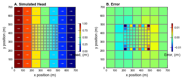
Run the USG1DISV model with XT3D, then plot heads.
[7]:
simulation(1)
<flopy.mf6.data.mfstructure.MFDataItemStructure object at 0x7f5513010190>
run_models took 13.02 ms