This page was generated from
ex-gwf-sfr-p01.py.
It's also available as a notebook.
Streamflow Routing Package Problem 1
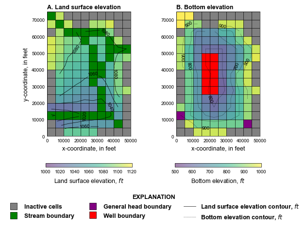
This is the stream-aquifer interaction example problem (test 1) from the Streamflow Routing Package documentation (Prudic, 1989). All reaches have been converted to rectangular reaches.
Initial setup
Import dependencies, define the example name and workspace, and read settings from environment variables.
[1]:
from pathlib import Path

import flopy
import git
import matplotlib as mpl
import matplotlib.pyplot as plt
import numpy as np
import pooch
from flopy.plot.styles import styles
from modflow_devtools.misc import get_env, timed

# Example name and workspace paths. If this example is running
# in the git repository, use the folder structure described in
# the README. Otherwise just use the current working directory.
sim_name = "ex-gwf-sfr-p01"
try:
    root = Path(git.Repo(".", search_parent_directories=True).working_dir)
except:
    root = None
workspace = root / "examples" if root else Path.cwd()
figs_path = root / "figures" if root else Path.cwd()
data_path = root / "data" / sim_name if root else Path.cwd()

# Settings from environment variables
write = get_env("WRITE", True)
run = get_env("RUN", True)
plot = get_env("PLOT", True)
plot_show = get_env("PLOT_SHOW", True)
plot_save = get_env("PLOT_SAVE", True)
Define parameters
Define model units, parameters and other settings.
[2]:
# Model units
length_units = "feet"
time_units = "seconds"

# Model parameters
nper = 3  # Number of periods
nlay = 1  # Number of layers
nrow = 15  # Number of rows
ncol = 10  # Number of columns
delr = 5000.0  # Column width ($ft$)
delc = 5000.0  # Row width ($ft$)
strt = 1050.0  # Starting head ($ft$)
k11_stream = 0.002  # Hydraulic conductivity near the stream ($ft/s$)
k11_basin = 0.0004  # Hydraulic conductivity in the basin ($ft/s$)
ss = 1e-6  # Specific storage ($1/s)$
sy_stream = 0.2  # Specific yield near the stream (unitless)
sy_basin = 0.1  # Specific yield in the basin (unitless)
evap_rate = 9.5e-8  # Evapotranspiration rate ($ft/s$)
ext_depth = 15.0  # Evapotranspiration extinction depth ($ft$)

# Time discretization
tdis_ds = (
    (0.0, 1, 1.0),
    (1.577880e9, 50, 1.1),
    (1.577880e9, 50, 1.1),
)

# Define dimensions
extents = (0.0, delr * ncol, 0.0, delc * nrow)
shape2d = (nrow, ncol)
shape3d = (nlay, nrow, ncol)

# Load the idomain, top, bottom, and evapotranspiration surface arrays
fname = "idomain.txt"
fpath = pooch.retrieve(
    url=f"https://github.com/MODFLOW-ORG/modflow6-examples/raw/master/data/{sim_name}/{fname}",
    fname=fname,
    path=data_path,
    known_hash="md5:a0b12472b8624aecdc79e5c19c97040c",
)
idomain = np.loadtxt(fpath, dtype=int)
fname = "top.txt"
fpath = pooch.retrieve(
    url=f"https://github.com/MODFLOW-ORG/modflow6-examples/raw/master/data/{sim_name}/{fname}",
    fname=fname,
    path=data_path,
    known_hash="md5:ab5097c1dc22e60fb313bf7f10dd8efe",
)
top = np.loadtxt(fpath, dtype=float)
fname = "bottom.txt"
fpath = pooch.retrieve(
    url=f"https://github.com/MODFLOW-ORG/modflow6-examples/raw/master/data/{sim_name}/{fname}",
    fname=fname,
    path=data_path,
    known_hash="md5:fa5fe276f4f58a01eabfe88516cc90af",
)
botm = np.loadtxt(fpath, dtype=float)
fname = "recharge.txt"
fpath = pooch.retrieve(
    url=f"https://github.com/MODFLOW-ORG/modflow6-examples/raw/master/data/{sim_name}/{fname}",
    fname=fname,
    path=data_path,
    known_hash="md5:82ed1ed29a457f1f38e51cd2657676e1",
)
recharge = np.loadtxt(fpath, dtype=float)
fname = "surf.txt"
fpath = pooch.retrieve(
    url=f"https://github.com/MODFLOW-ORG/modflow6-examples/raw/master/data/{sim_name}/{fname}",
    fname=fname,
    path=data_path,
    known_hash="md5:743ce03e5e46867cf5af94f1ac283514",
)
surf = np.loadtxt(fpath, dtype=float)

# Create hydraulic conductivity and specific yield
k11 = np.zeros(shape2d, dtype=float)
k11[idomain == 1] = k11_stream
k11[idomain == 2] = k11_basin
sy = np.zeros(shape2d, dtype=float)
sy[idomain == 1] = sy_stream
sy[idomain == 2] = sy_basin

# General head boundary conditions
ghb_spd = [
    [0, 12, 0, 988.0, 0.038],
    [0, 13, 8, 1045.0, 0.038],
]

# Well boundary conditions
wel_spd = {
    1: [
        [0, 5, 3, -10.0],
        [0, 5, 4, -10.0],
        [0, 6, 3, -10.0],
        [0, 6, 4, -10.0],
        [0, 7, 3, -10.0],
        [0, 7, 4, -10.0],
        [0, 8, 3, -10.0],
        [0, 8, 4, -10.0],
        [0, 9, 3, -10.0],
        [0, 9, 4, -10.0],
    ],
    2: [
        [],
    ],
}

# SFR Package
sfr_pakdata = [
    [0, 0, 0, 0, 4500.0, 12, 8.6767896e-04, 1093.048, 3.0, 0.00003, 0.030, 1, 1.0, 0],
    [1, 0, 1, 1, 7000.0, 12, 8.6767896e-04, 1088.059, 3.0, 0.00003, 0.030, 2, 1.0, 0],
    [2, 0, 2, 2, 6000.0, 12, 8.6767896e-04, 1082.419, 3.0, 0.00003, 0.030, 2, 1.0, 0],
    [3, 0, 2, 3, 5550.0, 12, 8.6767896e-04, 1077.408, 3.0, 0.00003, 0.030, 3, 1.0, 1],
    [4, 0, 3, 4, 6500.0, 12, 9.4339624e-04, 1071.934, 3.0, 0.00003, 0.030, 2, 1.0, 0],
    [5, 0, 4, 5, 5000.0, 12, 9.4339624e-04, 1066.509, 3.0, 0.00003, 0.030, 2, 1.0, 0],
    [6, 0, 5, 5, 5000.0, 12, 9.4339624e-04, 1061.792, 3.0, 0.00003, 0.030, 2, 1.0, 0],
    [7, 0, 6, 5, 5000.0, 12, 9.4339624e-04, 1057.075, 3.0, 0.00003, 0.030, 2, 1.0, 0],
    [8, 0, 7, 5, 5000.0, 12, 9.4339624e-04, 1052.359, 3.0, 0.00003, 0.030, 2, 1.0, 0],
    [9, 0, 2, 4, 5000.0, 10, 5.4545456e-04, 1073.636, 2.0, 0.00003, 0.030, 2, 0.0, 0],
    [10, 0, 2, 5, 5000.0, 10, 5.4545456e-04, 1070.909, 2.0, 0.00003, 0.030, 2, 1.0, 0],
    [11, 0, 2, 6, 4500.0, 10, 5.4545456e-04, 1068.318, 2.0, 0.00003, 0.030, 2, 1.0, 0],
    [12, 0, 3, 7, 6000.0, 10, 5.4545456e-04, 1065.455, 2.0, 0.00003, 0.030, 2, 1.0, 0],
    [13, 0, 4, 7, 5000.0, 10, 5.4545456e-04, 1062.455, 2.0, 0.00003, 0.030, 2, 1.0, 0],
    [14, 0, 5, 7, 2000.0, 10, 5.4545456e-04, 1060.545, 2.0, 0.00003, 0.030, 2, 1.0, 0],
    [15, 0, 4, 9, 2500.0, 10, 1.8181818e-03, 1077.727, 3.0, 0.00003, 0.030, 1, 1.0, 0],
    [16, 0, 4, 8, 5000.0, 10, 1.8181818e-03, 1070.909, 3.0, 0.00003, 0.030, 2, 1.0, 0],
    [17, 0, 5, 7, 3500.0, 10, 1.8181818e-03, 1063.182, 3.0, 0.00003, 0.030, 2, 1.0, 0],
    [18, 0, 5, 7, 4000.0, 15, 1.0000000e-03, 1058.000, 3.0, 0.00003, 0.030, 3, 1.0, 0],
    [19, 0, 6, 6, 5000.0, 15, 1.0000000e-03, 1053.500, 3.0, 0.00003, 0.030, 2, 1.0, 0],
    [20, 0, 7, 6, 3500.0, 15, 1.0000000e-03, 1049.250, 3.0, 0.00003, 0.030, 2, 1.0, 0],
    [21, 0, 7, 5, 2500.0, 15, 1.0000000e-03, 1046.250, 3.0, 0.00003, 0.030, 2, 1.0, 0],
    [22, 0, 8, 5, 5000.0, 12, 9.0909092e-04, 1042.727, 3.0, 0.00003, 0.030, 3, 1.0, 0],
    [23, 0, 9, 6, 5000.0, 12, 9.0909092e-04, 1038.182, 3.0, 0.00003, 0.030, 2, 1.0, 0],
    [24, 0, 10, 6, 5000.0, 12, 9.0909092e-04, 1033.636, 3.0, 0.00003, 0.030, 2, 1.0, 0],
    [25, 0, 11, 6, 5000.0, 12, 9.0909092e-04, 1029.091, 3.0, 0.00003, 0.030, 2, 1.0, 0],
    [26, 0, 12, 6, 2000.0, 12, 9.0909092e-04, 1025.909, 3.0, 0.00003, 0.030, 2, 1.0, 0],
    [27, 0, 13, 8, 5000.0, 55, 9.6774194e-04, 1037.581, 3.0, 0.00006, 0.025, 1, 1.0, 0],
    [28, 0, 12, 7, 5500.0, 55, 9.6774194e-04, 1032.500, 3.0, 0.00006, 0.025, 2, 1.0, 0],
    [29, 0, 12, 6, 5000.0, 55, 9.6774194e-04, 1027.419, 3.0, 0.00006, 0.025, 2, 1.0, 0],
    [30, 0, 12, 5, 5000.0, 40, 1.2500000e-03, 1021.875, 3.0, 0.00006, 0.025, 3, 1.0, 0],
    [31, 0, 12, 4, 5000.0, 40, 1.2500000e-03, 1015.625, 3.0, 0.00006, 0.025, 2, 1.0, 0],
    [32, 0, 12, 3, 5000.0, 40, 1.2500000e-03, 1009.375, 3.0, 0.00006, 0.025, 2, 1.0, 0],
    [33, 0, 12, 2, 5000.0, 40, 1.2500000e-03, 1003.125, 3.0, 0.00006, 0.025, 2, 1.0, 0],
    [34, 0, 12, 1, 5000.0, 40, 1.2500000e-03, 996.8750, 3.0, 0.00006, 0.025, 2, 1.0, 0],
    [35, 0, 12, 0, 3000.0, 40, 1.2500000e-03, 991.8750, 3.0, 0.00006, 0.025, 1, 1.0, 0],
]

sfr_conn = [
    [0, -1],
    [1, 0, -2],
    [2, 1, -3],
    [3, 2, -4, -9],
    [4, 3, -5],
    [5, 4, -6],
    [6, 5, -7],
    [7, 6, -8],
    [8, 7, -22],
    [9, 3, -10],
    [10, 9, -11],
    [11, 10, -12],
    [12, 11, -13],
    [13, 12, -14],
    [14, 13, -18],
    [15, -16],
    [16, 15, -17],
    [17, 16, -18],
    [18, 14, 17, -19],
    [19, 18, -20],
    [20, 19, -21],
    [21, 20, -22],
    [22, 8, 21, -23],
    [23, 22, -24],
    [24, 23, -25],
    [25, 24, -26],
    [26, 25, -30],
    [27, -28],
    [28, 27, -29],
    [29, 28, -30],
    [30, 26, 29, -31],
    [31, 30, -32],
    [32, 31, -33],
    [33, 32, -34],
    [34, 33, -35],
    [35, 34],
]

sfr_div = [[3, 0, 9, "UPTO"]]

sfr_spd = [
    [0, "inflow", 25.0],
    [15, "inflow", 10.0],
    [27, "inflow", 150.0],
    [3, "diversion", 0, 10.0],
    [9, "status", "simple"],
    [10, "status", "simple"],
    [11, "status", "simple"],
    [12, "status", "simple"],
    [13, "status", "simple"],
    [14, "status", "simple"],
    [9, "stage", 1075.545],
    [10, "stage", 1072.636],
    [11, "stage", 1069.873],
    [12, "stage", 1066.819],
    [13, "stage", 1063.619],
    [14, "stage", 1061.581],
]

# Solver parameters
nouter = 100
ninner = 50
hclose = 1e-6
rclose = 1e-6
Model setup
Define functions to build models, write input files, and run the simulation.
[3]:
def build_models():
    sim_ws = workspace / sim_name
    sim = flopy.mf6.MFSimulation(sim_name=sim_name, sim_ws=sim_ws, exe_name="mf6")
    flopy.mf6.ModflowTdis(sim, nper=nper, perioddata=tdis_ds, time_units=time_units)
    flopy.mf6.ModflowIms(
        sim,
        print_option="summary",
        linear_acceleration="bicgstab",
        outer_maximum=nouter,
        outer_dvclose=hclose,
        inner_maximum=ninner,
        inner_dvclose=hclose,
        rcloserecord=f"{rclose} strict",
    )
    gwf = flopy.mf6.ModflowGwf(
        sim, modelname=sim_name, newtonoptions="newton", save_flows=True
    )
    flopy.mf6.ModflowGwfdis(
        gwf,
        length_units=length_units,
        nlay=nlay,
        nrow=nrow,
        ncol=ncol,
        delr=delr,
        delc=delc,
        idomain=idomain,
        top=top,
        botm=botm,
    )
    flopy.mf6.ModflowGwfnpf(
        gwf,
        icelltype=1,
        k=k11,
        save_specific_discharge=True,
    )
    flopy.mf6.ModflowGwfsto(
        gwf,
        iconvert=1,
        sy=sy,
        ss=ss,
        steady_state={0: True},
        transient={1: True},
    )
    flopy.mf6.ModflowGwfic(gwf, strt=strt)
    flopy.mf6.ModflowGwfghb(gwf, stress_period_data=ghb_spd)
    flopy.mf6.ModflowGwfwel(gwf, stress_period_data=wel_spd)
    flopy.mf6.ModflowGwfrcha(gwf, recharge=recharge)
    flopy.mf6.ModflowGwfevta(gwf, surface=surf, rate=evap_rate, depth=ext_depth)
    sfr = flopy.mf6.ModflowGwfsfr(
        gwf,
        length_conversion=3.28081,
        nreaches=len(sfr_pakdata),
        packagedata=sfr_pakdata,
        connectiondata=sfr_conn,
        diversions=sfr_div,
        perioddata=sfr_spd,
    )
    obs_file = f"{sim_name}.sfr.obs"
    csv_file = obs_file + ".csv"
    obs_dict = {
        csv_file: [
            ("r01_stage", "stage", (3,)),
            ("r02_stage", "stage", (14,)),
            ("r03_stage", "stage", (26,)),
            ("r04_stage", "stage", (35,)),
            ("r01_flow", "downstream-flow", (3,)),
            ("r02_flow", "downstream-flow", (14,)),
            ("r03_flow", "downstream-flow", (26,)),
            ("r04_flow", "downstream-flow", (35,)),
        ]
    }
    sfr.obs.initialize(
        filename=obs_file, digits=10, print_input=True, continuous=obs_dict
    )

    head_filerecord = f"{sim_name}.hds"
    budget_filerecord = f"{sim_name}.cbc"
    flopy.mf6.ModflowGwfoc(
        gwf,
        head_filerecord=head_filerecord,
        budget_filerecord=budget_filerecord,
        saverecord=[("HEAD", "LAST"), ("BUDGET", "LAST")],
    )
    return sim


def write_models(sim, silent=True):
    sim.write_simulation(silent=silent)


@timed
def run_models(sim, silent=True):
    success, buff = sim.run_simulation(silent=silent)
    assert success, buff
Plotting results
Define functions to plot model results.
[4]:
# Figure properties
figure_size = (6.3, 5.6)
masked_values = (0, 1e30, -1e30)
def plot_grid(gwf, silent=True):
with styles.USGSMap() as fs:
fig = plt.figure(figsize=figure_size, constrained_layout=False)
gs = mpl.gridspec.GridSpec(ncols=10, nrows=7, figure=fig, wspace=5)
plt.axis("off")
axes = []
axes.append(fig.add_subplot(gs[:6, :5]))
axes.append(fig.add_subplot(gs[:6, 5:], sharey=axes[0]))
for ax in axes:
ax.set_xlim(extents[:2])
ax.set_ylim(extents[2:])
ax.set_aspect("equal")
# ax.set_xticks(ticklabels)
# ax.set_yticks(ticklabels)
# legend axis
axes.append(fig.add_subplot(gs[6:, :]))
# set limits for legend area
ax = axes[-1]
ax.set_xlim(0, 1)
ax.set_ylim(0, 1)
# get rid of ticks and spines for legend area
ax.axis("off")
ax.set_xticks([])
ax.set_yticks([])
ax.spines["top"].set_color("none")
ax.spines["bottom"].set_color("none")
ax.spines["left"].set_color("none")
ax.spines["right"].set_color("none")
ax.patch.set_alpha(0.0)
ax = axes[0]
mm = flopy.plot.PlotMapView(gwf, ax=ax, extent=extents)
top_coll = mm.plot_array(
top, vmin=1000, vmax=1120, masked_values=masked_values, alpha=0.5
)
mm.plot_bc("SFR", color="green")
cv = mm.contour_array(
top,
levels=np.arange(1000, 1100, 20),
linewidths=0.5,
linestyles="-",
colors="black",
masked_values=masked_values,
)
plt.clabel(cv, fmt="%1.0f")
mm.plot_inactive(color_noflow="0.5")
mm.plot_grid(lw=0.5, color="black")
cbar = plt.colorbar(
top_coll, shrink=0.8, orientation="horizontal", ax=ax, format="%.0f"
)
cbar.ax.tick_params(size=0)
cbar.ax.set_xlabel(r"Land surface elevation, $ft$")
ax.set_xlabel("x-coordinate, in feet")
ax.set_ylabel("y-coordinate, in feet")
styles.heading(ax, heading="Land surface elevation", idx=0)
styles.remove_edge_ticks(ax)
ax = axes[1]
mm = flopy.plot.PlotMapView(gwf, ax=ax, extent=extents)
bot_coll = mm.plot_array(
botm, vmin=500, vmax=1000, masked_values=masked_values, alpha=0.5
)
mm.plot_bc("GHB", color="purple")
mm.plot_bc("WEL", color="red", kper=1)
cv = mm.contour_array(
botm,
levels=np.arange(600, 1000, 100),
linewidths=0.5,
linestyles=":",
colors="black",
masked_values=masked_values,
)
plt.clabel(cv, fmt="%1.0f")
mm.plot_inactive(color_noflow="0.5")
mm.plot_grid(lw=0.5, color="black")
cbar = plt.colorbar(
bot_coll, shrink=0.8, orientation="horizontal", ax=ax, format="%.0f"
)
cbar.ax.tick_params(size=0)
cbar.ax.set_xlabel(r"Bottom elevation, $ft$")
ax.set_xlabel("x-coordinate, in feet")
styles.heading(ax, heading="Bottom elevation", idx=1)
styles.remove_edge_ticks(ax)
# legend
ax = axes[-1]
ax.plot(
-10000,
-10000,
lw=0,
marker="s",
ms=10,
mfc="0.5",
mec="black",
markeredgewidth=0.5,
label="Inactive cells",
)
ax.plot(
-10000,
-10000,
lw=0,
marker="s",
ms=10,
mfc="green",
mec="black",
markeredgewidth=0.5,
label="Stream boundary",
)
ax.plot(
-10000,
-10000,
lw=0,
marker="s",
ms=10,
mfc="purple",
mec="black",
markeredgewidth=0.5,
label="General head boundary",
)
ax.plot(
-10000,
-10000,
lw=0,
marker="s",
ms=10,
mfc="red",
mec="black",
markeredgewidth=0.5,
label="Well boundary",
)
ax.plot(
-10000,
-10000,
lw=0.5,
ls="-",
color="black",
label=r"Land surface elevation contour, $ft$",
)
ax.plot(
-10000,
-10000,
lw=0.5,
ls=":",
color="black",
label=r"Bottom elevation contour, $ft$",
)
styles.graph_legend(ax, loc="center", ncol=3)
if plot_show:
plt.show()
if plot_save:
fpth = figs_path / f"{sim_name}-grid.png"
fig.savefig(fpth)
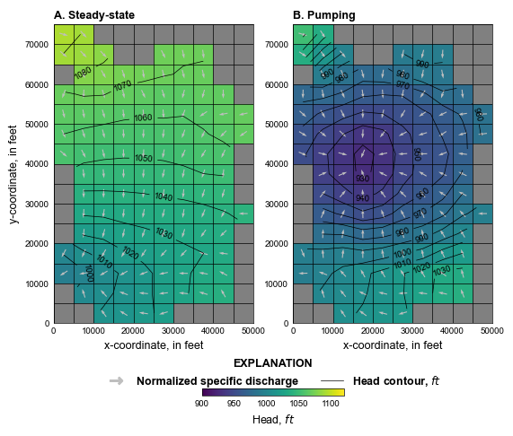
def plot_head_results(gwf, silent=True):
# create MODFLOW 6 head object
hobj = gwf.output.head()
# create MODFLOW 6 cell-by-cell budget object
cobj = gwf.output.budget()
kstpkper = hobj.get_kstpkper()
with styles.USGSMap():
fig = plt.figure(figsize=figure_size, constrained_layout=False)
gs = mpl.gridspec.GridSpec(ncols=10, nrows=7, figure=fig, wspace=5)
plt.axis("off")
axes = [fig.add_subplot(gs[:6, :5])]
axes.append(fig.add_subplot(gs[:6, 5:], sharey=axes[0]))
for ax in axes:
ax.set_xlim(extents[:2])
ax.set_ylim(extents[2:])
ax.set_aspect("equal")
# legend axis
axes.append(fig.add_subplot(gs[6:, :]))
# set limits for legend area
ax = axes[-1]
ax.set_xlim(0, 1)
ax.set_ylim(0, 1)
# get rid of ticks and spines for legend area
ax.axis("off")
ax.set_xticks([])
ax.set_yticks([])
ax.spines["top"].set_color("none")
ax.spines["bottom"].set_color("none")
ax.spines["left"].set_color("none")
ax.spines["right"].set_color("none")
ax.patch.set_alpha(0.0)
# extract heads and specific discharge for first stress period
head = hobj.get_data(kstpkper=kstpkper[0])
qx, qy, qz = flopy.utils.postprocessing.get_specific_discharge(
cobj.get_data(text="DATA-SPDIS", kstpkper=kstpkper[0])[0], gwf
)
ax = axes[0]
mm = flopy.plot.PlotMapView(gwf, ax=ax, extent=extents)
head_coll = mm.plot_array(
head, vmin=900, vmax=1120, masked_values=masked_values
)
cv = mm.contour_array(
head,
levels=np.arange(900, 1100, 10),
linewidths=0.5,
linestyles="-",
colors="black",
masked_values=masked_values,
)
plt.clabel(cv, fmt="%1.0f")
mm.plot_vector(qx, qy, normalize=True, color="0.75")
mm.plot_inactive(color_noflow="0.5")
mm.plot_grid(lw=0.5, color="black")
ax.set_xlabel("x-coordinate, in feet")
ax.set_ylabel("y-coordinate, in feet")
styles.heading(ax, heading="Steady-state", idx=0)
styles.remove_edge_ticks(ax)
# extract heads and specific discharge for second stress period
head = hobj.get_data(kstpkper=kstpkper[1])
qx, qy, qz = flopy.utils.postprocessing.get_specific_discharge(
cobj.get_data(text="DATA-SPDIS", kstpkper=kstpkper[1])[0], gwf
)
ax = axes[1]
mm = flopy.plot.PlotMapView(gwf, ax=ax, extent=extents)
head_coll = mm.plot_array(
head, vmin=900, vmax=1120, masked_values=masked_values
)
cv = mm.contour_array(
head,
levels=np.arange(900, 1100, 10),
linewidths=0.5,
linestyles="-",
colors="black",
masked_values=masked_values,
)
plt.clabel(cv, fmt="%1.0f")
mm.plot_vector(qx, qy, normalize=True, color="0.75")
mm.plot_inactive(color_noflow="0.5")
mm.plot_grid(lw=0.5, color="black")
ax.set_xlabel("x-coordinate, in feet")
styles.heading(ax, heading="Pumping", idx=1)
styles.remove_edge_ticks(ax)
# legend
ax = axes[-1]
cbar = plt.colorbar(
head_coll, shrink=0.8, orientation="horizontal", ax=ax, format="%.0f"
)
cbar.ax.tick_params(size=0)
cbar.ax.set_xlabel(r"Head, $ft$")
ax.plot(
-10000,
-10000,
lw=0,
marker="$\u2192$",
ms=10,
mfc="0.75",
mec="0.75",
label="Normalized specific discharge",
)
ax.plot(-10000, -10000, lw=0.5, color="black", label=r"Head contour, $ft$")
styles.graph_legend(ax, loc="upper center", ncol=2)
if plot_show:
plt.show()
if plot_save:
fpth = figs_path / f"{sim_name}-01.png"
fig.savefig(fpth)
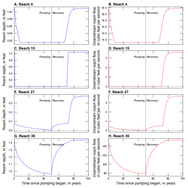
def plot_sfr_results(gwf, silent=True):
with styles.USGSPlot():
# load the observations
results = gwf.sfr.output.obs().data
# modify the time
results["totim"] /= 365.25 * 86400.0
rnos = (3, 14, 26, 35)
sfr = gwf.sfr.packagedata.array["rtp"]
offsets = []
for rno in rnos:
offsets.append(sfr[rno])
# create the figure
fig, axes = plt.subplots(
ncols=2, nrows=4, sharex=True, figsize=(6.3, 6.3), constrained_layout=True
)
ipos = 0
for i in range(4):
heading = f"Reach {rnos[i] + 1}"
for j in range(2):
ax = axes[i, j]
ax.set_xlim(0, 100)
if j == 0:
tag = f"R{i + 1:02d}_STAGE"
offset = offsets[i]
scale = 1.0
ylabel = "Reach depth, in feet"
color = "blue"
else:
tag = f"R{i + 1:02d}_FLOW"
offset = 0.0
scale = -1.0
ylabel = "Downstream reach flow,\nin cubic feet per second"
color = "red"
ax.plot(
results["totim"],
scale * results[tag] - offset,
lw=0.5,
color=color,
zorder=10,
)
ax.axvline(50, lw=0.5, ls="--", color="black", zorder=10)
if ax.get_ylim()[0] < 0.0:
ax.axhline(0, lw=0.5, color="0.5", zorder=9)
styles.add_text(
ax,
text="Pumping",
x=0.49,
y=0.8,
ha="right",
bold=False,
fontsize=7,
)
styles.add_text(
ax,
text="Recovery",
x=0.51,
y=0.8,
ha="left",
bold=False,
fontsize=7,
)
ax.set_ylabel(ylabel)
ax.yaxis.set_label_coords(-0.1, 0.5)
styles.heading(ax, heading=heading, idx=ipos)
if i == 3:
ax.set_xlabel("Time since pumping began, in years")
ipos += 1
if plot_show:
plt.show()
if plot_save:
fpth = figs_path / f"{sim_name}-02.png"
fig.savefig(fpth)
def plot_results(sim, silent=True):
gwf = sim.get_model(sim_name)
plot_grid(gwf, silent=silent)
plot_sfr_results(gwf, silent=silent)
plot_head_results(gwf, silent=silent)
Running the example
Define and invoke a function to run the example scenario, then plot results.
[5]:
def scenario(silent=True):
    sim = build_models()
    if write:
        write_models(sim, silent=silent)
    if run:
        run_models(sim, silent=silent)
    if plot:
        plot_results(sim, silent=silent)


# Simulated heads in model the unconfined, middle, and lower aquifers (model layers
# 1, 3, and 5) are shown in the figure below. MODFLOW-2005 results for a quasi-3D
# model are also shown. The location of drain (green) and well (gray) boundary
# conditions, normalized specific discharge, and head contours (25 ft contour
# intervals) are also shown.
scenario()
<flopy.mf6.data.mfstructure.MFDataItemStructure object at 0x7faa0c2d4f50>
run_models took 198.68 ms