USG1DISU example
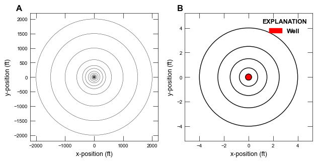
This example, ex-gwf-radial, shows how the MODFLOW 6 DISU Package can be used to simulate an axisymmetric radial model.
The example corresponds to the first example described in: Bedekar, V., Scantlebury, L., and Panday, S. (2019). Axisymmetric Modeling Using MODFLOW-USG.Groundwater, 57(5), 772-777.
And the numerical result is compared against the analytical solution presented in Equation 17 of Neuman, S. P. (1974). Effect of partial penetration on flow in unconfined aquifers considering delayed gravity response. Water resources research, 10(2), 303-312
Initial setup
Import dependencies, define the example name and workspace, and read settings from environment variables.
[1]:
import os
import pathlib as pl
from math import sqrt

import flopy
import git
import matplotlib.pyplot as plt
import numpy as np
from flopy.plot.styles import styles
from matplotlib.patches import Circle
from modflow_devtools.misc import get_env, timed

# Solve definite integral using Fortran library QUADPACK
from scipy.integrate import quad

# Find a root of a function using Brent's method within a bracketed range
from scipy.optimize import brentq

# Zero Order Bessel Function
from scipy.special import j0, jn_zeros

# Example name and workspace paths. If this example is running
# in the git repository, use the folder structure described in
# the README. Otherwise just use the current working directory.
sim_name = "ex-gwf-rad-disu"
try:
    root = pl.Path(git.Repo(".", search_parent_directories=True).working_dir)
except:
    root = None
workspace = root / "examples" if root else pl.Path.cwd()
figs_path = root / "figures" if root else pl.Path.cwd()

# Settings from environment variables
write = get_env("WRITE", True)
run = get_env("RUN", True)
plot = get_env("PLOT", True)
plot_show = get_env("PLOT_SHOW", True)
plot_save = get_env("PLOT_SAVE", True)
Define some utilities for creating the grid and solving the radial solution
[2]:
# Radial unconfined drawdown solution from Neuman 1974
pi = 3.141592653589793
sin = np.sin
cos = np.cos
sinh = np.sinh
cosh = np.cosh
exp = np.exp
def get_disu_radial_kwargs(
nlay,
nradial,
radius_outer,
surface_elevation,
layer_thickness,
get_vertex=False,
):
"""
Simple utility for creating radial unstructured elements
with the disu package.
Input assumes that each layer contains the same radial band,
but their thickness can be different.
Parameters
----------
nlay: number of layers (int)
nradial: number of radial bands to construct (int)
radius_outer: Outer radius of each radial band (array-like float with nradial length)
surface_elevation: Top elevation of layer 1 as either a float or nradial array-like float values.
If given as float, then value is replicated for each radial band.
layer_thickness: Thickness of each layer as either a float or nlay array-like float values.
If given as float, then value is replicated for each layer.
"""
pi = 3.141592653589793
def get_nn(lay, rad):
return nradial * lay + rad
def get_rad_array(var, rep):
try:
dim = len(var)
except:
dim, var = 1, [var]
if dim != 1 and dim != rep:
raise IndexError(
f"get_rad_array(var): var must be a scalar or have len(var)=={rep}"
)
if dim == 1:
return np.full(rep, var[0], dtype=np.float64)
else:
return np.array(var, dtype=np.float64)
nodes = nlay * nradial
surf = get_rad_array(surface_elevation, nradial)
thick = get_rad_array(layer_thickness, nlay)
iac = np.zeros(nodes, dtype=int)
ja = []
ihc = []
cl12 = []
hwva = []
area = np.zeros(nodes, dtype=float)
top = np.zeros(nodes, dtype=float)
bot = np.zeros(nodes, dtype=float)
for lay in range(nlay):
st = nradial * lay
sp = nradial * (lay + 1)
top[st:sp] = surf - thick[:lay].sum()
bot[st:sp] = surf - thick[: lay + 1].sum()
for lay in range(nlay):
for rad in range(nradial):
# diagonal/self
n = get_nn(lay, rad)
ja.append(n)
iac[n] += 1
if rad > 0:
area[n] = pi * (radius_outer[rad] ** 2 - radius_outer[rad - 1] ** 2)
else:
area[n] = pi * radius_outer[rad] ** 2
ihc.append(n + 1)
cl12.append(n + 1)
hwva.append(n + 1)
# up
if lay > 0:
ja.append(n - nradial)
iac[n] += 1
ihc.append(0)
cl12.append(0.5 * (top[n] - bot[n]))
hwva.append(area[n])
# to center
if rad > 0:
ja.append(n - 1)
iac[n] += 1
ihc.append(1)
cl12.append(0.5 * (radius_outer[rad] - radius_outer[rad - 1]))
hwva.append(2.0 * pi * radius_outer[rad - 1])
# to outer
if rad < nradial - 1:
ja.append(n + 1)
iac[n] += 1
ihc.append(1)
hwva.append(2.0 * pi * radius_outer[rad])
if rad > 0:
cl12.append(0.5 * (radius_outer[rad] - radius_outer[rad - 1]))
else:
cl12.append(radius_outer[rad])
# bottom
if lay < nlay - 1:
ja.append(n + nradial)
iac[n] += 1
ihc.append(0)
cl12.append(0.5 * (top[n] - bot[n]))
hwva.append(area[n])
# Build rectangular equivalent of radial coordinates (unwrap radial bands)
if get_vertex:
perimeter_outer = np.fromiter(
(2.0 * pi * rad for rad in radius_outer),
dtype=float,
count=nradial,
)
xc = 0.5 * radius_outer[0]
yc = 0.5 * perimeter_outer[-1]
# all cells have same y-axis cell center; yc is costant
#
# cell2d: [icell2d, xc, yc, ncvert, icvert]; first node: cell2d = [[0, xc, yc, [2, 1, 0]]]
cell2d = []
for lay in range(nlay):
n = get_nn(lay, 0)
cell2d.append([n, xc, yc, 3, 2, 1, 0])
#
xv = radius_outer[0]
# half perimeter is equal to the y shift for vertices
sh = 0.5 * perimeter_outer[0]
vertices = [
[0, 0.0, yc],
[1, xv, yc - sh],
[2, xv, yc + sh],
] # vertices: [iv, xv, yv]
iv = 3
for r in range(1, nradial):
# radius_outer[r-1] + 0.5*(radius_outer[r] - radius_outer[r-1])
xc = 0.5 * (radius_outer[r - 1] + radius_outer[r])
for lay in range(nlay):
n = get_nn(lay, r)
# cell2d: [icell2d, xc, yc, ncvert, icvert]
cell2d.append([n, xc, yc, 4, iv - 2, iv - 1, iv + 1, iv])
xv = radius_outer[r]
# half perimeter is equal to the y shift for vertices
sh = 0.5 * perimeter_outer[r]
vertices.append([iv, xv, yc - sh]) # vertices: [iv, xv, yv]
iv += 1
vertices.append([iv, xv, yc + sh]) # vertices: [iv, xv, yv]
iv += 1
cell2d.sort(key=lambda row: row[0]) # sort by node number
ja = np.array(ja, dtype=np.int32)
nja = ja.shape[0]
hwva = np.array(hwva, dtype=np.float64)
kw = {}
kw["nodes"] = nodes
kw["nja"] = nja
kw["nvert"] = None
kw["top"] = top
kw["bot"] = bot
kw["area"] = area
kw["iac"] = iac
kw["ja"] = ja
kw["ihc"] = ihc
kw["cl12"] = cl12
kw["hwva"] = hwva
if get_vertex:
kw["nvert"] = len(vertices) # = 2*nradial + 1
kw["vertices"] = vertices
kw["cell2d"] = cell2d
kw["angldegx"] = np.zeros(nja, dtype=float)
else:
kw["nvert"] = 0
return kw
def _find_hyperbolic_max_value():
seterr = np.seterr()
np.seterr(all="ignore")
inf = np.inf
x = 10.0
delt = 1.0
for i in range(1000000):
x += delt
try:
if inf == sinh(x):
break
except:
break
np.seterr(**seterr)
return x - delt
_hyperbolic_max_value = _find_hyperbolic_max_value()
def _find_hyperbolic_equivalent_value():
x = 10.0
delt = 0.0001
for i in range(1000000):
x += delt
if x > _hyperbolic_max_value:
break
try:
if sinh(x) == cosh(x):
return x
except:
break
return x - delt
_hyperbolic_equivalence = _find_hyperbolic_equivalent_value()
class RadialUnconfinedDrawdown:
"""
Solves the drawdown that occurs from pumping from partial penetration
in an unconfined, radial aquifer. Uses the method described in:
Neuman, S. P. (1974). Effect of partial penetration on flow in
unconfined aquifers considering delayed gravity response.
Water resources research, 10(2), 303-312.
"""
hyperbolic_max_value = _hyperbolic_max_value
hyperbolic_equivalence = _hyperbolic_equivalence
bottom: float
Kr: float
Kz: float
Ss: float
Sy: float
well_top: float
well_bot: float
saturated_thickness: float
_sigma: float
_beta: float
def __init__(
self,
bottom_elevation,
hydraulic_conductivity_radial=None,
hydraulic_conductivity_vertical=None,
specific_storage=None,
specific_yield=None,
well_screen_elevation_top=None,
well_screen_elevation_bottom=None,
water_table_elevation=None,
saturated_thickness=None,
):
"""
Initialize unconfined, radial groundwater model to solve drawdown
at an observation location in response to pumping at the center of
the model (that is, the well extracts water at radius = 0).
Parameters
----------
rad : int
radial band number (0 to nradial-1)
bottom_elevation : float
Elevation of the impermeable base of the model ($L$)
hydraulic_conductivity_radial : float
Radial direction hydraulic conductivity of model ($L/T$)
hydraulic_conductivity_vertical : float
Vertical (z) direction hydraulic conductivity of model ($L/T$)
specific_storage : float
Specific storage of aquifer ($1/T$)
specific_yield : float
Specific yield of aquifer ($-$)
well_screen_elevation_top : float
Pumping well's top screen elevation ($L$)
well_screen_elevation_bottom : float
Pumping well's bottom screen elevation ($L$)
water_table_elevation : float
Initial water table elevation. Note, saturated_thickness (b) is
calculated as $water_table_elevation - bottom_elevation$ ($L$)
saturated_thickness : float
Specify the initial saturated thickness of the unconfined aquifer.
Value is used to calculate the water_table_elevation. If
water_table_elevation is defined, then saturated_thickness input
is ignored and set to
$water_table_elevation - bottom_elevation$ ($L$)
"""
self.bottom = float(bottom_elevation)
self.Kr = self._float_or_none(hydraulic_conductivity_radial)
self.Kz = self._float_or_none(hydraulic_conductivity_vertical)
self.Ss = self._float_or_none(specific_storage)
self.Sy = self._float_or_none(specific_yield)
self.well_top = self._float_or_none(well_screen_elevation_top)
self.well_bot = self._float_or_none(well_screen_elevation_bottom)
if water_table_elevation is not None and saturated_thickness is not None:
raise RuntimeError(
"RadialUnconfinedDrawdown() must specify only "
+ "water_table_elevation or saturated_thickness, but not "
+ "both at the same time."
)
if water_table_elevation is not None:
self.saturated_thickness = float(water_table_elevation) - self.bottom
elif saturated_thickness is not None:
self.saturated_thickness = float(saturated_thickness)
else:
self.saturated_thickness = None
def _prop_check(self):
error = []
if self.Kr is None:
error.append("hydraulic_conductivity_radial")
if self.Kz is None:
error.append("hydraulic_conductivity_vertical")
if self.Ss is None:
error.append("specific_storage")
if self.Sy is None:
error.append("specific_yield")
if self.well_top is None:
error.append("well_screen_elevation_top")
if self.well_bot is None:
error.append("well_screen_elevation_bottom")
if error:
raise RuntimeError(
"RadialUnconfinedDrawdown: Attempted to solve radial "
+ "groundwater model\nwith the following input not specified\n"
+ "\n".join(error)
)
if self.well_top <= self.well_bot:
raise RuntimeError(
"RadialUnconfinedDrawdown: "
+ "well_screen_elevation_top <= well_screen_elevation_bottom\n"
+ f"That is: {self.well_top} <= "
+ f"{self.well_bot}"
)
def drawdown(
self,
pump,
time,
radius,
observation_elevation,
observation_elevation_bot=None,
sumrtol=1.0e-6,
u_n_rtol=1.0e-5,
epsabs=1.49e-8,
bessel_loop_limit=5,
quad_limit=128,
show_progress=False,
ty_time=False,
ts_time=False,
as_head=False,
):
"""
Solves the radial model's drawdown for a given pumping rate and
time at a given observation point
(radius, observation_elevation) or observation well screen interval
(radius, observation_elevation:observation_elevation_bot).
This solves drawdown by integrating equation 17 from
Neuman, S. P. (1974). Effect of partial penetration on flow in
unconfined aquifers considering delayed gravity response.
Water resources research, 10(2), 303-312
Parameters
----------
pump : float
Pumping rate of well at center of radial model ($L^3/T$)
Positive values are the water extraction rate.
Negative or zero values indicate no pumping and result returns
the dimensionless drawdown instead of regular drawdown.
time : float or Sequence[float]
Time that observation is made
radius : float
Radius of the observation location (distance from well, $L$)
observation_elevation : float
Either the location of the observation point, or the top elevation
of the observation well screen ($L$)
observation_elevation_bot : float
If specified, then represents the bottom elevation of the
observation well screen. If not specified (or set to None), then
observation location is treated as a single point, located at
radius and observation_elevation ($L$)
sumrtol : float
Solution involves integration of $y$ variable from 0 to ∞ from
Equation 17 in:
Neuman, S. P. (1974). Effect of partial penetration on flow in
unconfined aquifers considering delayed gravity response.
Water resources research, 10(2), 303-312.
The integration is broken into subsections that are spaced around
bessel function roots. The integration is complete when a
three sequential subsection solutions are less than
sumrtol times the largest subsection.
That is, the last included subsection contributes a
relatively small value compared to the largest of the sum.
u_n_rtol : float
Terminates the solution of the infinite series:
$\\sum_{n=1}^{\\infty} u_n(y)$
when
$u_n(y) < u_n(0) * u_n_rtol$
epsabs : float or int
scipy.integrate.quad absolute error tolerance.
Passed directly to that function's `epsabs` kwarg.
bessel_loop_limit : int
the integral is solved along each bessel function root.
The first 1024 roots are precalculated and automatically increased
if more are required. The upper limit for calculated roots is
1024 * 2 ^ bessel_loop_limit
If this limit is reached, then a warning is raised.
quad_limit : int
scipy.integrate.quad upper bound on the number of
subintervals used in the adaptive algorithm.
Passed directly to that function's `limit` kwarg.
show_progress : bool
if True, then progress is printed to the command prompt in the form:
ty_time : bool
if True, then `time` kwarg is dimensionless time with
respect to Specific Yield
ts_time : bool
if True, then `time` kwarg is dimensionless time with
respect to Specific Storage.
as_head : bool
If true, then drawdown result is converted to
head using the model bottom and initial saturated thickness.
If pump > 0, then as_head is ignored.
Returns
-------
result : float or list[float]
If time is float, then result is float.
If time is Sequence[float], then result is list[float].
If pump > 0, then result is the drawdown that occurs
from pump at time and radius at observation point
observation_elevation or from the observation well
screen interval observation_elevation to
observation_elevation_top ($L$).
If pump <= 0, then result is converted to
dimensionless drawdown ($-$)
"""
if not hasattr(time, "strip") and hasattr(time, "__iter__"):
return self.drawdown_times(
pump,
time,
radius,
observation_elevation,
observation_elevation_bot,
sumrtol,
u_n_rtol,
epsabs,
bessel_loop_limit,
quad_limit,
show_progress,
ty_time,
ts_time,
as_head,
)
return self.drawdown_times(
pump,
[time],
radius,
observation_elevation,
observation_elevation_bot,
sumrtol,
u_n_rtol,
epsabs,
bessel_loop_limit,
quad_limit,
show_progress,
ty_time,
ts_time,
as_head,
)[0]
def drawdown_times(
self,
pump,
times,
radius,
observation_elevation,
observation_elevation_bot=None,
sumrtol=1.0e-6,
u_n_rtol=1.0e-5,
epsabs=1.49e-8,
bessel_loop_limit=5,
quad_limit=128,
show_progress=False,
ty_time=False,
ts_time=False,
as_head=False,
):
# Same as self.drawdown, but times is a list[float] of
# observation times and returns a list[float] drawdowns.
if bessel_loop_limit < 1:
bessel_loop_limit = 1
bessel_roots0 = 1024
bessel_roots = bessel_roots0
bessel_root_limit_reached = []
self._prop_check()
if ty_time and ts_time:
raise RuntimeError(
"RadialUnconfinedDrawdown.drawdown_times "
+ "cannot set both ty_time and ts_time to True."
)
r = radius
b = self.saturated_thickness
sigma = self.Ss * b / self.Sy
beta = (r / b) * (r / b) * (self.Kz / self.Kr)
sqrt_beta = sqrt(beta)
if np.isnan(pump) or pump <= 0.0:
# Return dimensionless drawdown
coef = 1.0
else:
coef = pump / (4.0 * pi * b * self.Kr)
# dimensionless well screen top
dd = (self.saturated_thickness + self.bottom - self.well_top) / b
# dimensionless well screen bottom
ld = (self.saturated_thickness + self.bottom - self.well_bot) / b
# Solution must be in dimensionless time with respect to Ss;
# ts = kr*b*t/(Ss*b*r^2)
if ty_time:
ts_list = self.ty2ts(times)
elif ts_time:
ts_list = times
else:
ts_list = self.time2ts(times, r)
# distance above bottom to observation point or obs screen bottom
zt = observation_elevation - self.bottom
if observation_elevation_bot is None:
# Single Point Observation
zd = zt / b # dimensionless elevation of observation point
neuman1974_integral = self.neuman1974_integral1
obs_arg = (zd,)
else:
# distance above bottom to observation screen top
zb = observation_elevation_bot - self.bottom
# dimensionless elevation of observation screen interval
ztd, zbd = zt / b, zb / b
# dz = 1 / (zt - zb) -> implied in the
# modified u0 and uN functions
neuman1974_integral = self.neuman1974_integral2
obs_arg = (zbd, ztd)
s = [] # drawdown, one to one match with times
nstp = len(ts_list)
for stp, ts in enumerate(ts_list):
if show_progress:
print(
f"Solving {stp+1:4d} of {nstp}; " + f"time = {self.ts2time(ts, r)}",
end="",
)
args = (sigma, beta, sqrt_beta, ld, dd, ts, *obs_arg, u_n_rtol)
sol = 0.0
y0, y1 = 0.0, 0.0
mxdelt = 0.0
j0_roots = jn_zeros(0, bessel_roots) / sqrt_beta
jr0 = 0
jr1 = j0_roots.size
converged = 0
bessel_loop_count = 0
while converged < 3 and bessel_loop_count <= bessel_loop_limit:
if bessel_loop_count > 0:
bessel_roots *= 2
j0_roots = jn_zeros(0, bessel_roots) / sqrt_beta
jr0, jr1 = jr1, j0_roots.size
j0_roots_iter = np.nditer(j0_roots[jr0:jr1])
bessel_loop_count += 1
# Iterate over two roots to get full cycle
for j0_root in j0_roots_iter:
# First root
y0, y1 = y1, j0_root
delt1 = quad(
neuman1974_integral,
y0,
y1,
args,
epsabs=epsabs,
limit=quad_limit,
)[0]
#
# Second root
y0, y1 = y1, next(j0_roots_iter)
delt2 = quad(
neuman1974_integral,
y0,
y1,
args,
epsabs=epsabs,
limit=quad_limit,
)[0]
if np.isnan(delt1) or np.isnan(delt2):
break
sol += delt1 + delt2
adelt = abs(delt1 + delt2)
if adelt > mxdelt:
mxdelt = adelt
elif adelt < mxdelt * sumrtol:
converged += 1 # increment the convergence counter
# Converged if three sequential solutions (adelt)
# are less than mxdelt*sumrtol
if converged >= 3:
break
else:
converged = 0 # reset convergence counter
if sol < 0.0:
s.append(0.0)
else:
s.append(coef * sol)
if converged < 3:
bessel_root_limit_reached.append(stp)
if show_progress:
if converged < 3:
print(f"\ts = {s[-1]}\tbessel_loop_limit reached")
else:
print(f"\ts = {s[-1]}")
if pump > 0.0 and as_head:
initial_head = self.bottom + self.saturated_thickness
return [initial_head - drawdown for drawdown in s]
if len(bessel_root_limit_reached) > 0:
import warnings
root = j0_roots[-1]
bad_times = "\n".join([str(times[it]) for it in bessel_root_limit_reached])
warnings.warn(
"\n\nRadialUnconfinedDrawdown.drawdown_times failed to "
+ f"meet convergence sumrtol = {sumrtol}"
+ "\nwithin the precalculated Bessel root solutions "
+ "(convergence is evaluated at every second Bessel root).\n\n"
+ "The number of Bessel roots are automatically increased "
+ "up to:\n"
+ f" {bessel_roots0} * 2^bessel_loop_limit\nwhere:\n"
+ " bessel_loop_limit = {bessel_loop_limit}\n"
+ f"resulting in {1024*2**bessel_loop_limit} roots evaluated, "
+ "with the last root being {root}\n"
+ f"(That is, the Neuman integral was solved form 0 to {root})"
+ "\n\n"
+ "You can either ignore this warning\n"
+ "or to remove it attempt to increase bessel_loop_limit\n"
+ "or increase sumrtol (reducing accuracy).\n\nThe following "
+ "times are what triggered this warning:\n"
+ bad_times
+ "\n"
)
return s
@staticmethod
def neuman1974_integral1(y, alpha, beta, sqrt_beta, ld, dd, ts, zd, uN_tol=1.0e-6):
"""
Solves equation 17 from
Neuman, S. P. (1974). Effect of partial penetration on flow in
unconfined aquifers considering delayed gravity response.
Water resources research, 10(2), 303-312.
"""
if y == 0.0 or ts == 0.0:
return 0.0
u0 = RadialUnconfinedDrawdown.u_0(alpha, beta, zd, ld, dd, ts, y)
if np.isnan(u0):
u0 = 0.0
uN_func = RadialUnconfinedDrawdown.u_n
mxdelt = 0.0
uN = 0.0
for n in range(1, 25001):
delt = uN_func(alpha, beta, zd, ld, dd, ts, y, n)
if np.isnan(delt):
break
uN += delt
adelt = abs(delt)
if adelt > mxdelt:
mxdelt = adelt
elif adelt < mxdelt * uN_tol:
break
return 4.0 * y * j0(y * sqrt_beta) * (u0 + uN)
@staticmethod
def gamma0(g, y, s):
"""
Gamma0 root function from equation 18 in:
Neuman, S. P. (1974). Effect of partial penetration on flow in
unconfined aquifers considering delayed gravity response.
Water resources research, 10(2), 303-312.
=> Solution must be constrained by g^2 < y^2
To honor the constraint solution returns the absolute value
of the solution.
"""
if g >= _hyperbolic_equivalence:
# sinh ≈ cosh for large g
return s * g - (y * y - g * g)
return s * g * sinh(g) - (y * y - g * g) * cosh(g)
@staticmethod
def gammaN(g, y, s):
"""
GammaN root function from equation 19 in:
Neuman, S. P. (1974). Effect of partial penetration on flow in
unconfined aquifers considering delayed gravity response.
Water resources research, 10(2), 303-312.
=> Solution must be constrained by (2n-1)(π/2)< g < nπ
"""
return s * g * sin(g) + (y * y + g * g) * cos(g)
@staticmethod
def u_0(alpha, beta, z, l, d, ts, y):
gamma0 = RadialUnconfinedDrawdown.gamma0
a, b = 0.9 * y, y
try:
a, b = RadialUnconfinedDrawdown._get_bracket(gamma0, a, b, (y, alpha))
except RuntimeError:
a, b = RadialUnconfinedDrawdown._get_bracket(
gamma0, 0.0, b, (y, alpha), 1000
)
g = brentq(gamma0, a, b, args=(y, alpha), maxiter=500, xtol=1.0e-16)
# Check for cosh/sinh overflow
if g > _hyperbolic_max_value:
return 0.0
y2 = y * y
g2 = g * g
num1 = 1 - exp(-ts * beta * (y2 - g2))
num2 = cosh(g * z)
num3 = sinh(g * (1 - d)) - sinh(g * (1 - l))
den1 = y2 + (1 + alpha) * g2 - ((y2 - g2) ** 2) / alpha
den2 = cosh(g)
den3 = (l - d) * sinh(g)
# num1*num2*num3 / (den1*den2*den3)
return (num1 / den1) * (num2 / den2) * (num3 / den3)
@staticmethod
def u_n(alpha, beta, z, l, d, ts, y, n):
gammaN = RadialUnconfinedDrawdown.gammaN
a, b = (2 * n - 1) * (pi / 2.0), n * pi
try:
a, b = RadialUnconfinedDrawdown._get_bracket(gammaN, a, b, (y, alpha))
except RuntimeError:
a, b = RadialUnconfinedDrawdown._get_bracket(gammaN, a, b, (y, alpha), 1000)
g = brentq(gammaN, a, b, args=(y, alpha), maxiter=500, xtol=1.0e-16)
y2 = y * y
g2 = g * g
num1 = 1 - exp(-ts * beta * (y2 + g2))
num2 = cos(g * z)
num3 = sin(g * (1 - d)) - sin(g * (1 - l))
den1 = y2 - (1 + alpha) * g2 - ((y2 + g2) ** 2) / alpha
den2 = cos(g)
den3 = (l - d) * sin(g)
return num1 * num2 * num3 / (den1 * den2 * den3)
@staticmethod
def neuman1974_integral2(
y, alpha, beta, sqrt_beta, ld, dd, ts, z1, z2, uN_tol=1.0e-10
):
"""
Solves equation 20 from
Neuman, S. P. (1974). Effect of partial penetration on flow in
unconfined aquifers considering delayed gravity response.
Water resources research, 10(2), 303-312.
"""
if y == 0.0 or ts == 0.0:
return 0.0
u0 = RadialUnconfinedDrawdown.u_0_z1z2(alpha, beta, z1, z2, ld, dd, ts, y)
uN_func = RadialUnconfinedDrawdown.u_n_z1z2
mxdelt = 0.0
uN = 0.0
for n in range(1, 10001):
delt = uN_func(alpha, beta, z1, z2, ld, dd, ts, y, n)
uN += delt
adelt = abs(delt)
if adelt > mxdelt:
mxdelt = adelt
elif adelt < mxdelt * uN_tol:
break
return 4.0 * y * j0(y * sqrt_beta) * (u0 + uN)
@staticmethod
def u_0_z1z2(alpha, beta, z1, z2, l, d, ts, y):
gamma0 = RadialUnconfinedDrawdown.gamma0
a, b = 0.9 * y, y
try:
a, b = RadialUnconfinedDrawdown._get_bracket(gamma0, a, b, (y, alpha))
except RuntimeError:
a, b = RadialUnconfinedDrawdown._get_bracket(
gamma0, 0.0, b, (y, alpha), 1000
)
g = brentq(gamma0, a, b, args=(y, alpha), maxiter=500, xtol=1.0e-16)
# Check for cosh/sinh overflow
if g > _hyperbolic_max_value:
return 0.0
y2 = y * y
g2 = g * g
num1 = 1 - exp(-ts * beta * (y2 - g2))
num2 = sinh(g * z2) - sinh(g * z1)
num3 = sinh(g * (1 - d)) - sinh(g * (1 - l))
den1 = (y2 + (1 + alpha) * g2 - ((y2 - g2) ** 2) / alpha) * (z2 - z1) * g
den2 = cosh(g)
den3 = (l - d) * sinh(g)
# num1*num2*num3 / (den1*den2*den3)
return (num1 / den1) * (num2 / den2) * (num3 / den3)
@staticmethod
def u_n_z1z2(alpha, beta, z1, z2, l, d, ts, y, n):
gammaN = RadialUnconfinedDrawdown.gammaN
a, b = (2 * n - 1) * (pi / 2.0), n * pi
try:
a, b = RadialUnconfinedDrawdown._get_bracket(gammaN, a, b, (y, alpha))
except RuntimeError:
a, b = RadialUnconfinedDrawdown._get_bracket(gammaN, a, b, (y, alpha), 1000)
g = brentq(gammaN, a, b, args=(y, alpha), maxiter=500, xtol=1.0e-16)
y2 = y * y
g2 = g * g
num1 = 1 - exp(-ts * beta * (y2 + g2))
num2 = sin(g * z2) - sin(g * z1)
num3 = sin(g * (1 - d)) - sin(g * (1 - l))
den1 = y2 - (1 + alpha) * g2 - ((y2 + g2) ** 2) / alpha
den2 = cos(g) * (z2 - z1) * g
den3 = (l - d) * sin(g)
return num1 * num2 * num3 / (den1 * den2 * den3)
def time2ty(self, time, radius):
# dimensionless time with respect to Sy
if hasattr(time, "__iter__"):
# can iterate to get multiple times
return [
self.Kr * self.saturated_thickness * t / (self.Sy * radius * radius)
for t in time
]
return self.Kr * self.saturated_thickness * time / (self.Sy * radius * radius)
def time2ts(self, time, radius):
# dimensionless time with respect to Ss
if hasattr(time, "__iter__"):
# can iterate to get multiple times
return [self.Kr * t / (self.Ss * radius * radius) for t in time]
return self.Kr * time / (self.Ss * radius * radius)
def ty2time(self, ty, radius):
# dimensionless time with respect to Sy
if hasattr(ty, "__iter__"):
# can iterate to get multiple times
return [
t * self.Sy * radius * radius / (self.Kr * self.saturated_thickness)
for t in ty
]
return ty * self.Sy * radius * radius / (self.Kr * self.saturated_thickness)
def ts2time(self, ts, radius): # dimensionless time with respect to Ss
if hasattr(ts, "__iter__"): # can iterate to get multiple times
return [t * self.Ss * radius * radius / self.Kr for t in ts]
return ts * self.Ss * radius * radius / self.Kr
def ty2ts(self, ty):
if hasattr(ty, "__iter__"):
# can iterate to get multiple times
return [t * self.Sy / (self.Ss * self.saturated_thickness) for t in ty]
return ty * self.Sy / (self.Ss * self.saturated_thickness)
def drawdown2unitless(self, s, pump):
# dimensionless drawdown
return 4 * pi * self.Kr * self.saturated_thickness * s / pump
def unitless2drawdown(self, s, pump):
# drawdown
return pump * s / (4 * pi * self.Kr * self.saturated_thickness)
@staticmethod
def _float_or_none(val):
if val is not None:
return float(val)
return None
@staticmethod
def _get_bracket(func, a, b, arg=(), internal_search_split=100):
"""
Given initial range [a, b], search within the range for
root finding brackets.
That is, return [a, b] that results in f(a) * f(b) < 0.
"""
if a > b:
a, b = b, a
f1 = func(a, *arg)
f2 = func(b, *arg)
if f1 * f2 <= 0.0:
return a, b
# same sign, search within for sign change
delt = abs(b - a) / internal_search_split
a -= delt
for _ in range(internal_search_split):
a += delt
f1 = func(a, *arg)
if f1 * f2 <= 0.0:
return a, b
raise RuntimeError(
"get_bracket: failed to find bracket interval with opposite "
+ f"signs, that is: f(a)*f(b) < 0 for func: {func}"
)
def get_radial_node(rad, lay, nradial):
"""
Given nradial dimension (bands per layer),
returns the 0-based disu node number for given 0-based radial
band and layer
Parameters
----------
rad : int
radial band number (0 to nradial-1)
lay : float or ndarray
layer number (0 to nlay-1)
nradial : int
total number of radial bands
Returns
-------
result : int
0-based disu node number located at rad and lay
"""
return nradial * lay + rad
def get_radius_lay_from_node(node, nradial):
"""
Given nradial dimension (bands per layer),
returns 0-based layer and radial band indices for given disu node number
Parameters
----------
node : int
disu node number
nradial : int
total number of radial bands
Returns
-------
result : int
0-based disu node number located at rad and lay
"""
#
lay = node // nradial
rad = node - (lay * nradial)
return rad, lay
Define parameters
Define model units, parameters and other settings.
[3]:
# Model units
length_units = "feet"
time_units = "days"

# Model parameters
nper = 1  # Number of periods
_ = 24  # Number of time steps
_ = "10"  # Simulation total time ($day$)
nlay = 25  # Number of layers
nradial = 22  # Number of radial direction cells (radial bands)
initial_head = 50.0  # Initial water table elevation ($ft$)
surface_elevation = 50.0  # Top of the radial model ($ft$)
_ = 0.0  # Base of the radial model ($ft$)
layer_thickness = 2.0  # Thickness of each radial layer ($ft$)
_ = "0.25 to 2000"  # Outer radius of each radial band ($ft$)
k11 = 20.0  # Horizontal hydraulic conductivity ($ft/day$)
k33 = 20.0  # Vertical hydraulic conductivity ($ft/day$)
ss = 1.0e-5  # Specific storage ($1/day$)
sy = 0.1  # Specific yield (unitless)
_ = "0.0 to 10"  # Well screen elevation ($ft$)
_ = "1"  # Well radial band location (unitless)
_ = "-4000.0"  # Well pumping rate ($ft^3/day$)
_ = "40"  # Observation distance from well ($ft$)
_ = "1"  # ``Top'' observation elevation ($ft$)
_ = "25"  # ``Middle'' observation depth ($ft$)
_ = "49"  # ``Bottom'' observation depth ($ft$)


# Outer Radius for each radial band

radius_outer = [
    0.25,
    0.75,
    1.5,
    2.5,
    4.0,
    6.0,
    9.0,
    13.0,
    18.0,
    23.0,
    33.0,
    47.0,
    65.0,
    90.0,
    140.0,
    200.0,
    300.0,
    400.0,
    600.0,
    1000.0,
    1500.0,
    2000.0,
]  # Outer radius of each radial band ($ft$)

# Well boundary conditions
# Well must be located on central radial band (rad = 0)
# and have a contiguous screen interval and constant pumping rate.
# This example has the well screen interval from
# layer 20 to 24 (zero-based index)
wel_spd = {
    sp: [[(get_radial_node(0, lay, nradial),), -800.0] for lay in range(20, 25)]
    for sp in range(nper)
}

# Static temporal data used by TDIS file
# Simulation has 1 ten-day stress period with 24 time steps.
# The multiplier for the length of successive time steps is 1.62

tdis_ds = ((10.0, 24, 1.62),)

# Setup observation location and times

obslist = [
    ["h_top", "head", (get_radial_node(11, 0, nradial),)],
    ["h_mid", "head", (get_radial_node(11, (nlay - 1) // 2, nradial),)],
    ["h_bot", "head", (get_radial_node(11, nlay - 1, nradial),)],
]
obsdict = {"{}.obs.head.csv".format(sim_name): obslist}

# Solver parameters

nouter = 500
ninner = 300
hclose = 1e-4
rclose = 1e-4
Model setup
Define functions to build models, write input files, and run the simulation.
[4]:
def build_models(name):
    sim_ws = os.path.join(workspace, name)
    sim = flopy.mf6.MFSimulation(sim_name=name, sim_ws=sim_ws, exe_name="mf6")
    flopy.mf6.ModflowTdis(sim, nper=nper, perioddata=tdis_ds, time_units=time_units)
    flopy.mf6.ModflowIms(
        sim,
        print_option="summary",
        complexity="complex",
        outer_maximum=nouter,
        outer_dvclose=hclose,
        inner_maximum=ninner,
        inner_dvclose=hclose,
    )

    gwf = flopy.mf6.ModflowGwf(sim, modelname=name, save_flows=True)

    disukwargs = get_disu_radial_kwargs(
        nlay,
        nradial,
        radius_outer,
        surface_elevation,
        layer_thickness,
        get_vertex=True,
    )

    disu = flopy.mf6.ModflowGwfdisu(gwf, length_units=length_units, **disukwargs)

    npf = flopy.mf6.ModflowGwfnpf(
        gwf,
        k=k11,
        k33=k33,
        save_flows=True,
        save_specific_discharge=True,
    )

    flopy.mf6.ModflowGwfsto(
        gwf,
        iconvert=1,
        sy=sy,
        ss=ss,
        save_flows=True,
    )

    flopy.mf6.ModflowGwfic(gwf, strt=initial_head)

    flopy.mf6.ModflowGwfwel(gwf, stress_period_data=wel_spd, save_flows=True)

    flopy.mf6.ModflowGwfoc(
        gwf,
        budget_filerecord=f"{name}.cbc",
        head_filerecord=f"{name}.hds",
        headprintrecord=[("COLUMNS", nradial, "WIDTH", 15, "DIGITS", 6, "GENERAL")],
        saverecord=[("HEAD", "ALL"), ("BUDGET", "ALL")],
        printrecord=[("HEAD", "ALL"), ("BUDGET", "ALL")],
        filename=f"{name}.oc",
    )

    flopy.mf6.ModflowUtlobs(gwf, print_input=False, continuous=obsdict)
    return sim


def write_models(sim, silent=True):
    sim.write_simulation(silent=silent)


@timed
def run_models(sim, silent=True):
    success, buff = sim.run_simulation(silent=silent, report=True)
    assert success, buff
Plotting results
Define functions to plot model results.
[5]:
# Set default figure properties
figure_size = (6, 6)
def solve_analytical(obs2ana, times=None, no_solve=False):
"""Solve Axisymmetric model using analytical equation."""
# obs2ana = {obsdict[file][0] : analytical_name}
disukwargs = get_disu_radial_kwargs(
nlay, nradial, radius_outer, surface_elevation, layer_thickness
)
model_bottom = disukwargs["bot"][get_radial_node(0, nlay - 1, nradial)]
sat_thick = initial_head - model_bottom
key = next(iter(wel_spd))
nodes = []
rates = []
for nod, rat in wel_spd[key]:
nodes.append(nod[0])
rates.append(rat)
nodes.sort()
well_top = disukwargs["top"][nodes[0]]
well_bot = disukwargs["bot"][nodes[-1]]
pump = abs(sum(rates))
ana_model = RadialUnconfinedDrawdown(
bottom_elevation=model_bottom,
hydraulic_conductivity_radial=k11,
hydraulic_conductivity_vertical=k33,
specific_storage=ss,
specific_yield=sy,
well_screen_elevation_top=well_top,
well_screen_elevation_bottom=well_bot,
saturated_thickness=sat_thick,
)
build_times = times is None
if build_times:
totim = 0.0
for pertim in tdis_ds:
totim += pertim[0]
times_sy_base = np.logspace(-3, max([np.log10(totim), 2]), 100)
analytical = {}
prop = {}
if not no_solve:
print("Solving Analytical Model (Very Slow)")
for file in obsdict:
for row in obsdict[file]:
obs = row[0].upper()
if obs not in obs2ana:
continue
ana = obs2ana[obs]
nod = row[2][0]
obs_top = disukwargs["top"][nod]
obs_bot = disukwargs["bot"][nod]
rad, lay = get_radius_lay_from_node(nod, nradial)
if lay == 0:
# Uppermost layer has obs elevation at top,
# otherwise cell center
obs_el = obs_top
else:
obs_el = 0.5 * (obs_top + obs_bot)
if rad == 0:
obs_rad = 0.0
else:
# radius_outer[r-1] + 0.5*(radius_outer[r] - radius_outer[r-1])
obs_rad = 0.5 * (radius_outer[rad - 1] + radius_outer[rad])
if build_times:
times_sy = times_sy_base
times = [
ty * sy * obs_rad * obs_rad / (k11 * sat_thick)
for ty in times_sy_base
]
else:
times_sy = [
ty * k11 * sat_thick / (sy * obs_rad * obs_rad) for ty in times
]
times_ss = [ty * k11 / (ss * obs_rad * obs_rad) for ty in times]
if not no_solve:
print(f"Solving {ana}")
analytical[ana] = ana_model.drawdown_times(
pump,
times,
obs_rad,
obs_el,
sumrtol=1.0e-6,
u_n_rtol=1.0e-5,
)
prop[ana] = [
times,
times_sy,
times_ss,
pump,
obs_rad,
sat_thick,
model_bottom,
]
return analytical, prop
# Function to plot the Axisymmetric model results.
def plot_ts(sim, verbose=False, solve_analytical_solution=False):
pi = 3.141592653589793
gwf = sim.get_model(sim_name)
obs_csv_name = gwf.obs.output.obs_names[0]
obs_csv_file = gwf.obs.output.obs(f=obs_csv_name)
tsdata = obs_csv_file.data
fmt = {
"H_TOP": "og",
"H_MID": "or",
"H_BOT": "ob",
"a_top": "-g",
"a_mid": "-r",
"a_bot": "-b",
}
obsnames = {
"H_TOP": "MF6 (Top)",
"H_MID": "MF6 (Middle)",
"H_BOT": "MF6 (Bottom)",
"a_top": "Analytical (Top)",
"a_mid": "Analytical (Middle)",
"a_bot": "Analytical (Bottom)",
}
obs2ana = {"H_TOP": "a_top", "H_MID": "a_mid", "H_BOT": "a_bot"}
if solve_analytical_solution:
analytical, ana_prop = solve_analytical(obs2ana)
analytical_time = []
else:
analytical, ana_prop = solve_analytical(obs2ana, no_solve=True)
analytical_time = [
0.00016,
0.000179732,
0.000201897,
0.000226796,
0.000254765,
0.000286184,
0.000321477,
0.000361123,
0.000405658,
0.000455686,
0.000511883,
0.00057501,
0.000645923,
0.000725581,
0.000815062,
0.000915579,
0.001028492,
0.001155329,
0.001297809,
0.00145786,
0.00163765,
0.001839611,
0.002066479,
0.002321326,
0.002607601,
0.002929181,
0.00329042,
0.003696208,
0.004152039,
0.004664085,
0.005239279,
0.005885408,
0.00661122,
0.007426542,
0.008342413,
0.009371233,
0.010526932,
0.011825155,
0.013283481,
0.014921654,
0.016761852,
0.018828991,
0.021151058,
0.023759492,
0.026689609,
0.029981079,
0.033678466,
0.037831831,
0.042497405,
0.047738356,
0.053625642,
0.060238973,
0.067667886,
0.076012963,
0.085387188,
0.09591748,
0.107746411,
0.121034132,
0.13596055,
0.152727753,
0.171562756,
0.192720566,
0.216487644,
0.243185773,
0.273176424,
0.306865642,
0.34470955,
0.387220522,
0.434974119,
0.488616881,
0.548875086,
0.616564575,
0.692601805,
0.778016253,
0.873964355,
0.981745164,
1.102817937,
1.238821892,
1.391598404,
1.563215932,
1.755998025,
1.972554783,
2.215818194,
2.48908183,
2.79604544,
3.14086504,
3.528209184,
3.96332217,
4.452095044,
5.00114536,
5.617906775,
6.310729695,
7.088994332,
7.963237703,
8.945296292,
10.04846631,
11.2876837,
12.67972637,
14.24344137,
16,
]
analytical["a_top"] = [
9.14e-06,
1.48e-05,
2.32e-05,
3.51e-05,
5.16e-05,
7.39e-05,
0.000103386,
0.000141564,
0.000190115,
0.000250872,
0.000325813,
0.000417056,
0.00052686,
0.000657611,
0.000811829,
0.000992179,
0.001201482,
0.001442755,
0.001719253,
0.002034538,
0.002392557,
0.002797739,
0.003255095,
0.003770324,
0.004349925,
0.005001299,
0.005732852,
0.006554096,
0.007475752,
0.008509865,
0.009669933,
0.010971051,
0.01243007,
0.014065786,
0.015899134,
0.017953402,
0.020254465,
0.022831026,
0.025714866,
0.028941104,
0.032548456,
0.03657948,
0.041080814,
0.046103371,
0.051702489,
0.057938,
0.064874212,
0.072579742,
0.081127182,
0.090592554,
0.101054493,
0.112593132,
0.125288641,
0.139219391,
0.154459742,
0.171077492,
0.189131034,
0.208666373,
0.229714163,
0.252287007,
0.276377285,
0.301955794,
0.328971456,
0.357352252,
0.387007461,
0.417831084,
0.449706211,
0.482509951,
0.516118451,
0.550411552,
0.585276682,
0.620611726,
0.656326766,
0.692344745,
0.72860122,
0.765043446,
0.801629049,
0.838324511,
0.875103648,
0.911946208,
0.94883664,
0.985763066,
1.022716447,
1.059689924,
1.0966783,
1.133677645,
1.170684993,
1.207698108,
1.24471531,
1.281735341,
1.318757264,
1.355780385,
1.392804192,
1.429828316,
1.466852493,
1.503876535,
1.540900317,
1.577923757,
1.614946805,
1.651969438,
]
analytical["a_mid"] = [
0.042573248,
0.053215048,
0.065047371,
0.077900907,
0.091562277,
0.10578645,
0.120308736,
0.134861006,
0.149179898,
0.163017203,
0.176149026,
0.188382628,
0.199562503,
0.209575346,
0.218353885,
0.22587733,
0.232171831,
0.237306589,
0.241387585,
0.244548545,
0.246940521,
0.24872049,
0.250040497,
0.25103848,
0.251831919,
0.252514802,
0.253157938,
0.253811816,
0.254511215,
0.255280058,
0.256135833,
0.257093057,
0.258165369,
0.259366956,
0.260713168,
0.262220999,
0.263909262,
0.265798794,
0.267912645,
0.270276262,
0.272917675,
0.27586768,
0.279160018,
0.28283153,
0.286922294,
0.291475727,
0.296538626,
0.302161152,
0.308396727,
0.31530182,
0.322935596,
0.331359479,
0.340636352,
0.350829851,
0.362003212,
0.374217985,
0.387532593,
0.402000693,
0.417669407,
0.434577538,
0.452753827,
0.472215504,
0.492966953,
0.514999008,
0.538288679,
0.562799606,
0.588483025,
0.615279515,
0.643120962,
0.671933085,
0.701637983,
0.732156526,
0.763410706,
0.795325415,
0.827829825,
0.860858334,
0.894351053,
0.928253957,
0.962518747,
0.997102451,
1.031967356,
1.067080013,
1.102411044,
1.137934722,
1.17362841,
1.209472238,
1.245448747,
1.281542585,
1.317740238,
1.354029805,
1.390400789,
1.426843932,
1.463351049,
1.499914938,
1.53652918,
1.573188127,
1.609886766,
1.64662066,
1.683385875,
1.720178921,
]
analytical["a_bot"] = [
0.086684154,
0.103649206,
0.12188172,
0.141163805,
0.16124535,
0.181846061,
0.202667182,
0.223392774,
0.243699578,
0.263275092,
0.281824849,
0.299088528,
0.31485153,
0.328955429,
0.341304221,
0.351868481,
0.360684432,
0.367848506,
0.373508853,
0.377853369,
0.381094083,
0.383450902,
0.385136877,
0.386345028,
0.387238663,
0.387947536,
0.388568938,
0.389170336,
0.389796684,
0.390476869,
0.39123089,
0.392073081,
0.393015962,
0.39407278,
0.395256673,
0.396583156,
0.398068337,
0.399731151,
0.401591476,
0.403672105,
0.405997893,
0.408596189,
0.411497001,
0.414733164,
0.418340479,
0.422357833,
0.426826999,
0.431793796,
0.437306073,
0.443415589,
0.450176656,
0.457646089,
0.46588273,
0.47494648,
0.484898814,
0.495799471,
0.507707617,
0.520679174,
0.534765662,
0.550012634,
0.566458073,
0.584130854,
0.60304937,
0.623219948,
0.644638018,
0.667285046,
0.691130674,
0.716132499,
0.742239678,
0.76939134,
0.797520861,
0.826557513,
0.85642935,
0.887062398,
0.918386519,
0.950334816,
0.982842103,
1.015851071,
1.049306941,
1.083160734,
1.117368294,
1.151890127,
1.186690934,
1.221739246,
1.257007172,
1.292471077,
1.32810677,
1.363895877,
1.399822391,
1.435868577,
1.472023401,
1.508273605,
1.544607161,
1.581017341,
1.617494414,
1.654030939,
1.690620311,
1.72725511,
1.763933202,
1.800648435,
]
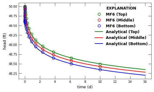
with styles.USGSPlot() as fs:
obs_fig = "obs-head"
fig = plt.figure(figsize=(5, 3))
ax = fig.add_subplot()
ax.set_xlabel("time (d)")
ax.set_ylabel("head (ft)")
for name in tsdata.dtype.names[1:]:
ax.plot(
tsdata["totim"],
tsdata[name],
fmt[name],
label=obsnames[name],
markerfacecolor="none",
)
# , markersize=3
for name in analytical:
n = len(analytical[name])
if solve_analytical_solution:
ana_times = ana_prop[name][0]
else:
ana_times = analytical_time
ax.plot(
ana_times[:n],
[50.0 - h for h in analytical[name]],
fmt[name],
label=obsnames[name],
)
styles.graph_legend(ax)
fig.tight_layout()
if plot_save:
fpth = figs_path / "{}-{}{}".format(sim_name, obs_fig, ".png")
fig.savefig(fpth)
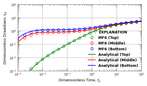
obs_fig = "obs-dimensionless"
fig = plt.figure(figsize=(5, 3))
fig.tight_layout()
ax = fig.add_subplot()
ax.set_xlim(0.001, 100.0)
ax.set_ylim(0.001, 100.0)
ax.grid(visible=True, which="major", axis="both")
ax.set_ylabel("Dimensionless Drawdown, $s_d$")
ax.set_xlabel("Dimensionless Time, $t_y$")
for name in tsdata.dtype.names[1:]:
q = ana_prop[obs2ana[name]][3]
r = ana_prop[obs2ana[name]][4]
b = ana_prop[obs2ana[name]][5]
ax.loglog(
[k11 * b * ts / (sy * r * r) for ts in tsdata["totim"]],
[4 * pi * k11 * b * (initial_head - h) / q for h in tsdata[name]],
fmt[name],
label=obsnames[name],
markerfacecolor="none",
)
for name in analytical:
q = ana_prop[name][3]
b = ana_prop[name][5] # [pump, radius, sat_thick, model_bottom]
if solve_analytical_solution:
ana_times = ana_prop[name][0]
else:
ana_times = analytical_time
n = len(analytical[name])
time_sy = [k11 * b * ts / (sy * r * r) for ts in ana_times[:n]]
ana = [4 * pi * k11 * b * s / q for s in analytical[name]]
ax.plot(time_sy, ana, fmt[name], label=obsnames[name])
styles.graph_legend(ax)
fig.tight_layout()
if plot_save:
fpth = figs_path / "{}-{}{}".format(sim_name, obs_fig, ".png")
fig.savefig(fpth)
# Function to plot the model radial bands.
def plot_grid(verbose=False):
with styles.USGSMap():
# Print all radial bands
fig, axs = plt.subplots(nrows=1, ncols=2, figsize=(6.4, 3.1))
# fig, axs = plt.subplots(nrows=1, ncols=2, figsize=(10, 4.5))
ax = axs[0]
max_rad = radius_outer[-1]
max_rad = max_rad + (max_rad * 0.1)
ax.set_xlim(-max_rad, max_rad)
ax.set_ylim(-max_rad, max_rad)
ax.set_aspect("equal", adjustable="box")
circle_center = (0.0, 0.0)
for r in radius_outer:
circle = Circle(circle_center, r, color="black", fill=False, lw=0.3)
ax.add_artist(circle)
ax.set_xlabel("x-position (ft)")
ax.set_ylabel("y-position (ft)")
ax.annotate(
"A",
(-0.11, 1.02),
xycoords="axes fraction",
fontweight="black",
fontsize="xx-large",
)
# Print first 5 radial bands
nband = 5
ax = axs[1]
radius_subset = radius_outer[:nband]
max_rad = radius_subset[-1]
max_rad = max_rad + (max_rad * 0.3)
ax.set_xlim(-max_rad, max_rad)
ax.set_ylim(-max_rad, max_rad)
ax.set_aspect("equal", adjustable="box")
circle_center = (0.0, 0.0)
r = radius_subset[0]
circle = Circle(circle_center, r, color="red", label="Well")
ax.add_artist(circle)
for r in radius_subset:
circle = Circle(circle_center, r, color="black", lw=1, fill=False)
ax.add_artist(circle)
ax.set_xlabel("x-position (ft)")
ax.set_ylabel("y-position (ft)")
ax.annotate(
"B",
(-0.06, 1.02),
xycoords="axes fraction",
fontweight="black",
fontsize="xx-large",
)
styles.graph_legend(ax)
fig.tight_layout()
if plot_show:
plt.show()
if plot_save:
fpth = figs_path / "{}-grid{}".format(sim_name, ".png")
fig.savefig(fpth)
# Function to plot the model results.
def plot_results(silent=True):
if not plot:
return
if silent:
verbosity_level = 0
else:
verbosity_level = 1
sim_ws = os.path.join(workspace, sim_name)
sim = flopy.mf6.MFSimulation.load(
sim_name=sim_name, sim_ws=sim_ws, verbosity_level=verbosity_level
)
verbose = not silent
# If True, solves the Neuman 1974 analytical model (very slow)
# else uses stored results from solving the Neuman 1974 analytical model
analytical = False
plot_grid(verbose)
plot_ts(sim, verbose, solve_analytical_solution=analytical)
Running the example
Define and invoke a function to run the example scenario, then plot results.
[6]:
def scenario(silent=True):
    # key = list(parameters.keys())[idx]
    # params = parameters[key].copy()
    sim = build_models(sim_name)
    if write:
        write_models(sim, silent=silent)
    if run:
        run_models(sim, silent=silent)


# MF6 Axisymmetric Model
scenario()

if plot:
    # Solve analytical and plot results with MF6 results
    plot_results()
run_models took 123.71 ms