This page was generated from
ex-gwf-lak-p01.py.
It's also available as a notebook.
Lake Package Problem 1
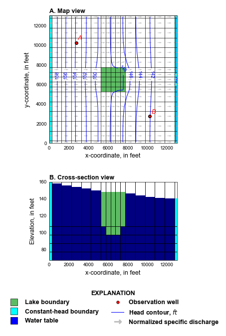
This is the lake package example problem (test 1) from the Lake Package documentation (Merritt and Konikow, 2000).
Initial setup
Import dependencies, define the example name and workspace, and read settings from environment variables.
[1]:
from pathlib import Path

import flopy
import git
import matplotlib.pyplot as plt
import numpy as np
from flopy.plot.styles import styles
from modflow_devtools.misc import get_env, timed

# Example name and workspace paths. If this example is running
# in the git repository, use the folder structure described in
# the README. Otherwise just use the current working directory.
sim_name = "ex-gwf-lak-p01"
try:
    root = Path(git.Repo(".", search_parent_directories=True).working_dir)
except:
    root = None
workspace = root / "examples" if root else Path.cwd()
figs_path = root / "figures" if root else Path.cwd()

# Settings from environment variables
write = get_env("WRITE", True)
run = get_env("RUN", True)
plot = get_env("PLOT", True)
plot_show = get_env("PLOT_SHOW", True)
plot_save = get_env("PLOT_SAVE", True)
Define parameters
Define model units, parameters and other settings.
[2]:
# Model units
length_units = "feet"
time_units = "days"

# Model parameters
nper = 1  # Number of periods
nlay = 5  # Number of layers
nrow = 17  # Number of rows
ncol = 17  # Number of columns
top = 500.0  # Top of the model ($ft$)
botm_str = "107., 97., 87., 77., 67."  # Bottom elevations ($ft$)
strt = 115.0  # Starting head ($ft$)
k11 = 30.0  # Horizontal hydraulic conductivity ($ft/d$)
k33_str = "1179., 30., 30., 30., 30."  # Vertical hydraulic conductivity ($ft/d$)
ss = 3e-4  # Specific storage ($1/d$)
sy = 0.2  # Specific yield (unitless)
H1 = 160.0  # Constant head on left side of model ($ft$)
H2 = 140.0  # Constant head on right side of model ($ft$)
recharge = 0.0116  # Aereal recharge rate ($ft/d$)
etvrate = 0.0141  # Maximum evapotranspiration rate ($ft/d$)
etvdepth = 15.0  # Evapotranspiration extinction depth ($ft$)
lak_strt = 110.0  # Starting lake stage ($ft$)
lak_etrate = 0.0103  # Lake evaporation rate ($ft/d$)
lak_bedleak = 0.1  # Lakebed leakance ($1/d$)

# parse parameter strings into tuples
botm = [float(value) for value in botm_str.split(",")]
k33 = [float(value) for value in k33_str.split(",")]

# Static temporal data used by TDIS file
tdis_ds = ((5000.0, 100, 1.02),)

# define delr and delc
delr = np.array(
    [
        250.0,
        1000.0,
        1000.0,
        1000.0,
        1000.0,
        1000.0,
        500.00,
        500.00,
        500.00,
        500.0,
        500.00,
        1000.0,
        1000.0,
        1000.0,
        1000.0,
        1000.0,
        250.0,
    ]
)
delc = np.array(
    [
        250.0,
        1000.0,
        1000.0,
        1000.0,
        1000.0,
        1000.0,
        500.00,
        500.00,
        500.00,
        500.0,
        500.00,
        1000.0,
        1000.0,
        1000.0,
        1000.0,
        1000.0,
        250.0,
    ]
)

# Define dimensions
extents = (0.0, delr.sum(), 0.0, delc.sum())
shape2d = (nrow, ncol)
shape3d = (nlay, nrow, ncol)

# Create the array defining the lake location
lake_map = np.ones(shape3d, dtype=np.int32) * -1
lake_map[0, 6:11, 6:11] = 0
lake_map[1, 7:10, 7:10] = 0
lake_map = np.ma.masked_where(lake_map < 0, lake_map)

# create linearly varying evapotranspiration surface
xlen = delr.sum() - 0.5 * (delr[0] + delr[-1])
x = 0.0
s1d = H1 * np.ones(ncol, dtype=float)
for idx in range(1, ncol):
    x += 0.5 * (delr[idx - 1] + delr[idx])
    frac = x / xlen
    s1d[idx] = H1 + (H2 - H1) * frac
surf = np.tile(s1d, (nrow, 1))
surf[lake_map[0] == 0] = botm[0] - 2
surf[lake_map[1] == 0] = botm[1] - 2

# Constant head boundary conditions
chd_spd = []
for k in range(nlay):
    chd_spd += [[k, i, 0, H1] for i in range(nrow)]
    chd_spd += [[k, i, ncol - 1, H2] for i in range(nrow)]

# LAK Package
lak_spd = [
    [0, "rainfall", recharge],
    [0, "evaporation", lak_etrate],
]

# Solver parameters
nouter = 500
ninner = 100
hclose = 1e-9
rclose = 1e-6
Model setup
Define functions to build models, write input files, and run the simulation.
[3]:
def build_models():
    sim_ws = workspace / sim_name
    sim = flopy.mf6.MFSimulation(sim_name=sim_name, sim_ws=sim_ws, exe_name="mf6")
    flopy.mf6.ModflowTdis(sim, nper=nper, perioddata=tdis_ds, time_units=time_units)
    flopy.mf6.ModflowIms(
        sim,
        print_option="summary",
        linear_acceleration="bicgstab",
        outer_maximum=nouter,
        outer_dvclose=hclose,
        inner_maximum=ninner,
        inner_dvclose=hclose,
        rcloserecord=f"{rclose} strict",
    )
    gwf = flopy.mf6.ModflowGwf(
        sim, modelname=sim_name, newtonoptions="newton", save_flows=True
    )
    flopy.mf6.ModflowGwfdis(
        gwf,
        length_units=length_units,
        nlay=nlay,
        nrow=nrow,
        ncol=ncol,
        delr=delr,
        delc=delc,
        idomain=np.ones(shape3d, dtype=int),
        top=top,
        botm=botm,
    )
    obs_file = f"{sim_name}.gwf.obs"
    csv_file = obs_file + ".csv"
    obslist = [
        ["A", "head", (0, 3, 3)],
        ["B", "head", (0, 13, 13)],
    ]
    obsdict = {csv_file: obslist}
    flopy.mf6.ModflowUtlobs(
        gwf, filename=obs_file, print_input=False, continuous=obsdict
    )

    flopy.mf6.ModflowGwfnpf(
        gwf,
        icelltype=1,
        k=k11,
        k33=k33,
        save_specific_discharge=True,
    )
    flopy.mf6.ModflowGwfsto(
        gwf,
        iconvert=1,
        sy=sy,
        ss=ss,
    )
    flopy.mf6.ModflowGwfic(gwf, strt=strt)
    flopy.mf6.ModflowGwfchd(gwf, stress_period_data=chd_spd)
    flopy.mf6.ModflowGwfrcha(gwf, recharge=recharge)
    flopy.mf6.ModflowGwfevta(gwf, surface=surf, rate=etvrate, depth=etvdepth)
    (idomain_wlakes, pakdata_dict, lak_conn) = flopy.mf6.utils.get_lak_connections(
        gwf.modelgrid, lake_map, bedleak=lak_bedleak
    )
    lak_packagedata = [[0, lak_strt, pakdata_dict[0]]]
    lak = flopy.mf6.ModflowGwflak(
        gwf,
        print_stage=True,
        nlakes=1,
        noutlets=0,
        packagedata=lak_packagedata,
        connectiondata=lak_conn,
        perioddata=lak_spd,
    )
    obs_file = f"{sim_name}.lak.obs"
    csv_file = obs_file + ".csv"
    obs_dict = {
        csv_file: [
            ("stage", "stage", (0,)),
        ]
    }
    lak.obs.initialize(
        filename=obs_file, digits=10, print_input=True, continuous=obs_dict
    )
    gwf.dis.idomain = idomain_wlakes

    head_filerecord = f"{sim_name}.hds"
    budget_filerecord = f"{sim_name}.cbc"
    flopy.mf6.ModflowGwfoc(
        gwf,
        head_filerecord=head_filerecord,
        budget_filerecord=budget_filerecord,
        saverecord=[("HEAD", "LAST"), ("BUDGET", "LAST")],
    )
    return sim


def write_models(sim, silent=True):
    sim.write_simulation(silent=silent)


@timed
def run_models(sim, silent=True):
    success, buff = sim.run_simulation(silent=silent)
    assert success, buff
Model setup
Define functions to build models, write input files, and run the simulation.
[4]:
# Figure properties
figure_size = (6.3, 5.6)
masked_values = (0, 1e30, -1e30)
def plot_grid(gwf, silent=True):
# load the observations
lak_results = gwf.lak.output.obs().data
# create MODFLOW 6 head object
hobj = gwf.output.head()
# create MODFLOW 6 cell-by-cell budget object
cobj = gwf.output.budget()
kstpkper = hobj.get_kstpkper()
head = hobj.get_data(kstpkper=kstpkper[0])
qx, qy, qz = flopy.utils.postprocessing.get_specific_discharge(
cobj.get_data(text="DATA-SPDIS", kstpkper=kstpkper[0])[0], gwf
)
# add lake stage to heads
head[head == 1e30] = lak_results["STAGE"][-1]
# observation locations
xcenters, ycenters = gwf.modelgrid.xycenters[0], gwf.modelgrid.xycenters[1]
p1 = (xcenters[3], ycenters[3])
p2 = (xcenters[13], ycenters[13])
with styles.USGSMap():
fig = plt.figure(figsize=(4, 6.9), tight_layout=True)
plt.axis("off")
nrows, ncols = 10, 1
axes = [fig.add_subplot(nrows, ncols, (1, 5))]
axes.append(fig.add_subplot(nrows, ncols, (6, 8), sharex=axes[0]))
for idx, ax in enumerate(axes):
ax.set_xlim(extents[:2])
if idx == 0:
ax.set_ylim(extents[2:])
ax.set_aspect("equal")
# legend axis
axes.append(fig.add_subplot(nrows, ncols, (9, 10)))
# set limits for legend area
ax = axes[-1]
ax.set_xlim(0, 1)
ax.set_ylim(0, 1)
# get rid of ticks and spines for legend area
ax.axis("off")
ax.set_xticks([])
ax.set_yticks([])
ax.spines["top"].set_color("none")
ax.spines["bottom"].set_color("none")
ax.spines["left"].set_color("none")
ax.spines["right"].set_color("none")
ax.patch.set_alpha(0.0)
ax = axes[0]
mm = flopy.plot.PlotMapView(gwf, ax=ax, extent=extents)
mm.plot_bc("CHD", color="cyan")
mm.plot_inactive(color_noflow="#5DBB63")
mm.plot_grid(lw=0.5, color="black")
cv = mm.contour_array(
head,
levels=np.arange(140, 160, 2),
linewidths=0.75,
linestyles="-",
colors="blue",
masked_values=masked_values,
)
plt.clabel(cv, fmt="%1.0f")
mm.plot_vector(qx, qy, normalize=True, color="0.75")
ax.plot(p1[0], p1[1], marker="o", mfc="red", mec="black", ms=4)
ax.plot(p2[0], p2[1], marker="o", mfc="red", mec="black", ms=4)
ax.set_xlabel("x-coordinate, in feet")
ax.set_ylabel("y-coordinate, in feet")
styles.heading(ax, heading="Map view", idx=0)
styles.add_text(
ax,
"A",
x=p1[0] + 150,
y=p1[1] + 150,
transform=False,
bold=False,
color="red",
ha="left",
va="bottom",
)
styles.add_text(
ax,
"B",
x=p2[0] + 150,
y=p2[1] + 150,
transform=False,
bold=False,
color="red",
ha="left",
va="bottom",
)
styles.remove_edge_ticks(ax)
ax = axes[1]
xs = flopy.plot.PlotCrossSection(gwf, ax=ax, line={"row": 8})
xs.plot_array(np.ones(shape3d), head=head, cmap="jet")
xs.plot_bc("CHD", color="cyan", head=head)
xs.plot_ibound(color_noflow="#5DBB63", head=head)
xs.plot_grid(lw=0.5, color="black")
ax.set_xlabel("x-coordinate, in feet")
ax.set_ylim(67, 160)
ax.set_ylabel("Elevation, in feet")
styles.heading(ax, heading="Cross-section view", idx=1)
styles.remove_edge_ticks(ax)
# legend
ax = axes[-1]
ax.plot(
-10000,
-10000,
lw=0,
marker="s",
ms=10,
mfc="#5DBB63",
mec="black",
markeredgewidth=0.5,
label="Lake boundary",
)
ax.plot(
-10000,
-10000,
lw=0,
marker="s",
ms=10,
mfc="cyan",
mec="black",
markeredgewidth=0.5,
label="Constant-head boundary",
)
ax.plot(
-10000,
-10000,
lw=0,
marker="s",
ms=10,
mfc="blue",
mec="black",
markeredgewidth=0.5,
label="Water table",
)
ax.plot(
-10000,
-10000,
lw=0,
marker="o",
ms=4,
mfc="red",
mec="black",
markeredgewidth=0.5,
label="Observation well",
)
ax.plot(
-10000, -10000, lw=0.75, ls="-", color="blue", label=r"Head contour, $ft$"
)
ax.plot(
-10000,
-10000,
lw=0,
marker="$\u2192$",
ms=10,
mfc="0.75",
mec="0.75",
label="Normalized specific discharge",
)
styles.graph_legend(ax, loc="lower center", ncol=2)
if plot_show:
plt.show()
if plot_save:
fpth = figs_path / f"{sim_name}-grid.png"
fig.savefig(fpth)
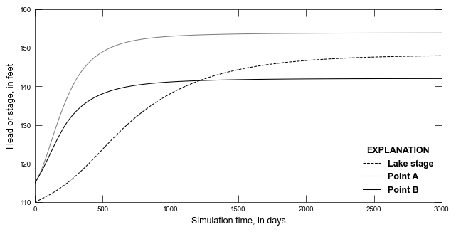
def plot_lak_results(gwf, silent=True):
with styles.USGSPlot():
# load the observations
lak_results = gwf.lak.output.obs().data
gwf_results = gwf.obs[0].output.obs().data
dtype = [
("time", float),
("STAGE", float),
("A", float),
("B", float),
]
results = np.zeros((lak_results.shape[0] + 1), dtype=dtype)
results["time"][1:] = lak_results["totim"]
results["STAGE"][0] = 110.0
results["STAGE"][1:] = lak_results["STAGE"]
results["A"][0] = 115.0
results["A"][1:] = gwf_results["A"]
results["B"][0] = 115.0
results["B"][1:] = gwf_results["B"]
# create the figure
fig, ax = plt.subplots(
ncols=1, nrows=1, sharex=True, figsize=(6.3, 3.15), constrained_layout=True
)
ax.set_xlim(0, 3000)
ax.set_ylim(110, 160)
ax.plot(
results["time"],
results["STAGE"],
lw=0.75,
ls="--",
color="black",
label="Lake stage",
)
ax.plot(
results["time"], results["A"], lw=0.75, ls="-", color="0.5", label="Point A"
)
ax.plot(
results["time"],
results["B"],
lw=0.75,
ls="-",
color="black",
label="Point B",
)
ax.set_xlabel("Simulation time, in days")
ax.set_ylabel("Head or stage, in feet")
styles.graph_legend(ax, loc="lower right")
if plot_show:
plt.show()
if plot_save:
fpth = figs_path / f"{sim_name}-01.png"
fig.savefig(fpth)
def plot_results(sim, silent=True):
gwf = sim.get_model(sim_name)
plot_grid(gwf, silent=silent)
plot_lak_results(gwf, silent=silent)
Running the example
Define and invoke a function to run the example scenario, then plot results.
[5]:
def scenario(silent=True):
    sim = build_models()
    if write:
        write_models(sim, silent=silent)
    if run:
        run_models(sim, silent=silent)
    if plot:
        plot_results(sim, silent=silent)


scenario()
<flopy.mf6.data.mfstructure.MFDataItemStructure object at 0x7fa2a8bb8050>
run_models took 7593.08 ms