This page was generated from ex-gwf-hani.py. It's also available as a notebook.

Hani example

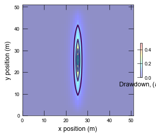
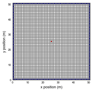
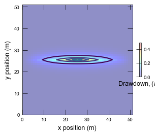
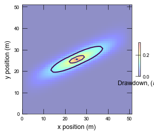
Simple steady state model using a regular MODFLOW grid to simulate the response of an anisotropic confined aquifer to a pumping well. A constant-head boundary condition surrounds the active domain. K22 is set to 0.01. Drawdown is more pronounced in the K11 direction.

Initial setup

Import dependencies, define the example name and workspace, and read settings from environment variables.

import os
import pathlib as pl

import flopy
import flopy.utils.cvfdutil
import git
import matplotlib.pyplot as plt
import numpy as np
from flopy.plot.styles import styles
from modflow_devtools.misc import get_env, timed

# Example name and workspace paths. If this example is running
# in the git repository, use the folder structure described in
# the README. Otherwise just use the current working directory.
try:
    root = pl.Path(git.Repo(".", search_parent_directories=True).working_dir)
except:
    root = None
workspace = root / "examples" if root else pl.Path.cwd()
figs_path = root / "figures" if root else pl.Path.cwd()

# Settings from environment variables
write = get_env("WRITE", True)
run = get_env("RUN", True)
plot = get_env("PLOT", True)
plot_show = get_env("PLOT_SHOW", True)
plot_save = get_env("PLOT_SAVE", True)

Define parameters

Define model units, parameters and other settings.

# Model units
length_units = "meters"
time_units = "days"

# Scenario-specific parameters
parameters = {
    "ex-gwf-hanir": {"angle1": 0, "xt3d": False},
    "ex-gwf-hanix": {"angle1": 25, "xt3d": True},
    "ex-gwf-hanic": {"angle1": 90, "xt3d": False},
}

# Model parameters
nper = 1  # Number of periods
nlay = 1  # Number of layers
nrow = 51  # Number of rows
ncol = 51  # Number of columns
delr = 10.0  # Spacing along rows ($m$)
delc = 10.0  # Spacing along columns ($m$)
top = 0.0  # Top of the model ($m$)
botm = -10.0  # Layer bottom elevations ($m$)
strt = 0.0  # Starting head ($m$)
icelltype = 0  # Cell conversion type
k11 = 1.0  # Horizontal hydraulic conductivity in the 11 direction ($m/d$)
k22 = 0.01  # Horizontal hydraulic conductivity in the 22 direction ($m/d$)
pumping_rate = -1.0  # Pumping rate ($m^3/d$)

# Static temporal data used by TDIS file
# Simulation has 1 steady stress period (1 day)

perlen = [1.0]
nstp = [1]
tsmult = [1.0]
tdis_ds = list(zip(perlen, nstp, tsmult))

nouter = 50
ninner = 100
hclose = 1e-9
rclose = 1e-6

Model setup

Define functions to build models, write input files, and run the simulation.

def build_models(sim_name, angle1, xt3d):
    sim_ws = os.path.join(workspace, sim_name)
    sim = flopy.mf6.MFSimulation(sim_name=sim_name, sim_ws=sim_ws, exe_name="mf6")
    flopy.mf6.ModflowTdis(sim, nper=nper, perioddata=tdis_ds, time_units=time_units)
    flopy.mf6.ModflowIms(
        sim,
        linear_acceleration="bicgstab",
        outer_maximum=nouter,
        outer_dvclose=hclose,
        inner_maximum=ninner,
        inner_dvclose=hclose,
        rcloserecord=f"{rclose} strict",
    )
    gwf = flopy.mf6.ModflowGwf(sim, modelname=sim_name, save_flows=True)
    flopy.mf6.ModflowGwfdis(
        gwf,
        length_units=length_units,
        nlay=nlay,
        nrow=nrow,
        ncol=ncol,
        top=top,
        botm=botm,
    )
    flopy.mf6.ModflowGwfnpf(
        gwf,
        icelltype=icelltype,
        k=k11,
        k22=k22,
        angle1=angle1,
        save_specific_discharge=True,
        xt3doptions=xt3d,
    )
    flopy.mf6.ModflowGwfic(gwf, strt=strt)

    ibd = -1 * np.ones((nrow, ncol), dtype=int)
    ibd[1:-1, 1:-1] = 1
    chdrow, chdcol = np.where(ibd == -1)
    chd_spd = [[0, i, j, 0.0] for i, j in zip(chdrow, chdcol)]
    flopy.mf6.ModflowGwfchd(
        gwf,
        stress_period_data=chd_spd,
        pname="CHD",
    )
    flopy.mf6.ModflowGwfwel(
        gwf,
        stress_period_data=[0, 25, 25, pumping_rate],
        pname="WEL",
    )
    head_filerecord = f"{sim_name}.hds"
    budget_filerecord = f"{sim_name}.cbc"
    flopy.mf6.ModflowGwfoc(
        gwf,
        head_filerecord=head_filerecord,
        budget_filerecord=budget_filerecord,
        saverecord=[("HEAD", "ALL"), ("BUDGET", "ALL")],
    )

    return sim


def write_models(sim, silent=True):
    sim.write_simulation(silent=silent)


@timed
def run_models(sim, silent=False):
    success, buff = sim.run_simulation(silent=silent, report=True)
    assert success, buff

Plotting results

Define functions to plot model results.

# Set default figure properties
figure_size = (3.5, 3.5)


def plot_grid(idx, sim):
    with styles.USGSMap():
        sim_name = list(parameters.keys())[idx]
        sim_ws = os.path.join(workspace, sim_name)
        gwf = sim.get_model(sim_name)

        fig = plt.figure(figsize=figure_size)
        fig.tight_layout()

        ax = fig.add_subplot(1, 1, 1, aspect="equal")
        pmv = flopy.plot.PlotMapView(model=gwf, ax=ax, layer=0)
        pmv.plot_grid()
        pmv.plot_bc(name="CHD")
        pmv.plot_bc(name="WEL")
        ax.set_xlabel("x position (m)")
        ax.set_ylabel("y position (m)")

        if plot_show:
            plt.show()
        if plot_save:
            fpth = figs_path / f"{sim_name}-grid.png"
            fig.savefig(fpth)


def plot_head(idx, sim):
    with styles.USGSMap():
        sim_name = list(parameters.keys())[idx]
        sim_ws = os.path.join(workspace, sim_name)
        gwf = sim.get_model(sim_name)

        fig = plt.figure(figsize=figure_size)
        fig.tight_layout()

        head = gwf.output.head().get_data()

        ax = fig.add_subplot(1, 1, 1, aspect="equal")
        pmv = flopy.plot.PlotMapView(model=gwf, ax=ax, layer=0)
        cb = pmv.plot_array(0 - head, cmap="jet", alpha=0.25)
        cs = pmv.contour_array(0 - head, levels=np.arange(0.1, 1, 0.1))
        cbar = plt.colorbar(cb, shrink=0.25)
        cbar.ax.set_xlabel(r"Drawdown, ($m$)")
        ax.set_xlabel("x position (m)")
        ax.set_ylabel("y position (m)")

        if plot_show:
            plt.show()
        if plot_save:
            fpth = figs_path / f"{sim_name}-head.png"
            fig.savefig(fpth)


def plot_results(idx, sim, silent=True):
    if idx == 0:
        plot_grid(idx, sim)
    plot_head(idx, sim)

Running the example

Define and invoke a function to run the example scenario, then plot results.

def scenario(idx, silent=True):
    key = list(parameters.keys())[idx]
    params = parameters[key].copy()
    sim = build_models(key, **params)
    if write:
        write_models(sim, silent=silent)
    if run:
        run_models(sim, silent=silent)
    if plot:
        plot_results(idx, sim, silent=silent)


# Run the Hani model with anisotropy in x direction and plot heads.

scenario(0)

# Run the Hani model with anisotropy in y direction and plot heads.

scenario(1)

# Run the Hani model with anisotropy rotated 15 degrees and plot heads.

scenario(2)

<flopy.mf6.data.mfstructure.MFDataItemStructure object at 0x7f649fc61ee0>
run_models took 44.48 ms

<flopy.mf6.data.mfstructure.MFDataItemStructure object at 0x7f649fc61ee0>
run_models took 62.28 ms

<flopy.mf6.data.mfstructure.MFDataItemStructure object at 0x7f649fc61ee0>
run_models took 45.58 ms