This page was generated from
ex-gwf-fhb.py.
It's also available as a notebook.
Flow and Head Boundary (FHB) Package Replication
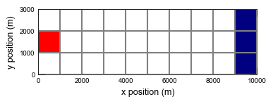
This example shows how the time series capability in MODFLOW 6 can be combined with the constant head and well packages to replicate the functionality of the Flow and Head Boundary (FHB) Package in previous versions of MODFLOW.
Initial setup
Import dependencies, define the example name and workspace, and read settings from environment variables.
[1]:
from pathlib import Path

import flopy
import git
import matplotlib.pyplot as plt
from flopy.plot.styles import styles
from modflow_devtools.misc import get_env, timed

# Example name and workspace paths. If this example is running
# in the git repository, use the folder structure described in
# the README. Otherwise just use the current working directory.
sim_name = "ex-gwf-fhb"
try:
    root = Path(git.Repo(".", search_parent_directories=True).working_dir)
except:
    root = None
workspace = root / "examples" if root else Path.cwd()
figs_path = root / "figures" if root else Path.cwd()

# Settings from environment variables
write = get_env("WRITE", True)
run = get_env("RUN", True)
plot = get_env("PLOT", True)
plot_show = get_env("PLOT_SHOW", True)
plot_save = get_env("PLOT_SAVE", True)
Define parameters
Define model units, parameters and other settings.
[2]:
# Model units
length_units = "meters"
time_units = "days"

# Model parameters
nper = 3  # Number of periods
nlay = 1  # Number of layers
ncol = 10  # Number of columns
nrow = 3  # Number of rows
delr = 1000.0  # Column width ($m$)
delc = 1000.0  # Row width ($m$)
top = 50.0  # Top of the model ($m$)
botm_str = "-200.0"  # Layer bottom elevations ($m$)
strt = 0.0  # Starting head ($m$)
icelltype_str = "0"  # Cell conversion type
k11_str = "20.0"  # Horizontal hydraulic conductivity ($m/d$)
ss = 0.01  # Specific storage ($/m$)

# Static temporal data used by TDIS file
# Simulation has 1 steady stress period (1 day)
# and 3 transient stress periods (10 days each).
# Each transient stress period has 120 2-hour time steps.
perlen = [400.0, 200.0, 400.0]
nstp = [10, 4, 6]
tsmult = [1.0, 1.0, 1.0]
tdis_ds = list(zip(perlen, nstp, tsmult))

# Parse parameter strings into tuples
botm = [float(value) for value in botm_str.split(",")]
k11 = [float(value) for value in k11_str.split(",")]
icelltype = [int(value) for value in icelltype_str.split(",")]

# Solver parameters
nouter = 50
ninner = 100
hclose = 1e-9
rclose = 1e-6
Model setup
Define functions to build models, write input files, and run the simulation.
[3]:
def build_models():
    sim_ws = workspace / sim_name
    sim = flopy.mf6.MFSimulation(sim_name=sim_name, sim_ws=sim_ws, exe_name="mf6")
    flopy.mf6.ModflowTdis(sim, nper=nper, perioddata=tdis_ds, time_units=time_units)
    flopy.mf6.ModflowIms(
        sim,
        outer_maximum=nouter,
        outer_dvclose=hclose,
        inner_maximum=ninner,
        inner_dvclose=hclose,
        rcloserecord=f"{rclose} strict",
    )
    gwf = flopy.mf6.ModflowGwf(sim, modelname=sim_name, save_flows=True)
    flopy.mf6.ModflowGwfdis(
        gwf,
        length_units=length_units,
        nlay=nlay,
        nrow=nrow,
        ncol=ncol,
        delr=delr,
        delc=delc,
        top=top,
        botm=botm,
    )
    flopy.mf6.ModflowGwfnpf(
        gwf,
        icelltype=icelltype,
        k=k11,
        save_specific_discharge=True,
    )
    flopy.mf6.ModflowGwfic(gwf, strt=strt)
    flopy.mf6.ModflowGwfsto(
        gwf,
        storagecoefficient=True,
        iconvert=0,
        ss=1.0e-6,
        sy=None,
        transient={0: True},
    )

    chd_spd = []
    chd_spd += [[0, i, 9, "CHDHEAD"] for i in range(3)]
    chd_spd = {0: chd_spd}
    tsdata = [(0.0, 0.0), (307.0, 1.0), (791.0, 5.0), (1000.0, 2.0)]
    tsdict = {
        "timeseries": tsdata,
        "time_series_namerecord": "CHDHEAD",
        "interpolation_methodrecord": "LINEAREND",
    }
    flopy.mf6.ModflowGwfchd(
        gwf,
        stress_period_data=chd_spd,
        timeseries=tsdict,
        pname="CHD",
    )

    wel_spd = []
    wel_spd += [[0, 1, 0, "FLOWRATE"]]
    wel_spd = {0: wel_spd}
    tsdata = [
        (0.0, 2000.0),
        (307.0, 6000.0),
        (791.0, 5000.0),
        (1000.0, 9000.0),
    ]
    tsdict = {
        "timeseries": tsdata,
        "time_series_namerecord": "FLOWRATE",
        "interpolation_methodrecord": "LINEAREND",
    }
    flopy.mf6.ModflowGwfwel(
        gwf,
        stress_period_data=wel_spd,
        timeseries=tsdict,
        pname="WEL",
    )

    head_filerecord = f"{sim_name}.hds"
    budget_filerecord = f"{sim_name}.cbc"
    flopy.mf6.ModflowGwfoc(
        gwf,
        head_filerecord=head_filerecord,
        budget_filerecord=budget_filerecord,
        saverecord=[("HEAD", "ALL"), ("BUDGET", "ALL")],
    )

    obsdict = {}
    obslist = [
        ["h1_2_1", "head", (0, 1, 0)],
        ["h1_2_10", "head", (0, 1, 9)],
    ]
    obsdict[f"{sim_name}.obs.head.csv"] = obslist
    obslist = [["icf1", "flow-ja-face", (0, 1, 1), (0, 1, 0)]]
    obsdict[f"{sim_name}.obs.flow.csv"] = obslist
    obs = flopy.mf6.ModflowUtlobs(gwf, print_input=False, continuous=obsdict)

    return sim


def write_models(sim, silent=True):
    sim.write_simulation(silent=silent)


@timed
def run_models(sim, silent=False):
    success, buff = sim.run_simulation(silent=silent, report=True)
    assert success, buff
Plotting results
Define functions to plot model results.
[4]:
# Figure properties
figure_size = (4, 4)
def plot_grid(sim):
with styles.USGSMap():
gwf = sim.get_model(sim_name)
fig = plt.figure(figsize=(4, 3.0))
fig.tight_layout()
ax = fig.add_subplot(1, 1, 1, aspect="equal")
pmv = flopy.plot.PlotMapView(model=gwf, ax=ax, layer=0)
pmv.plot_grid()
pmv.plot_bc(name="CHD")
pmv.plot_bc(name="WEL")
ax.set_xlabel("x position (m)")
ax.set_ylabel("y position (m)")
if plot_show:
plt.show()
if plot_save:
fpth = figs_path / f"{sim_name}-grid.png"
fig.savefig(fpth)
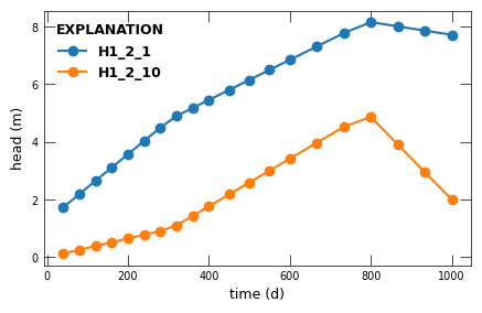
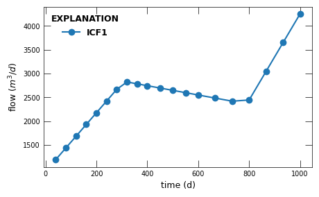
def plot_ts(sim):
with styles.USGSPlot():
gwf = sim.get_model(sim_name)
obsnames = gwf.obs.output.obs_names
obs_list = [
gwf.obs.output.obs(f=obsnames[0]),
gwf.obs.output.obs(f=obsnames[1]),
]
ylabel = ["head (m)", "flow ($m^3/d$)"]
obs_fig = ("obs-head", "obs-flow", "ghb-obs")
for iplot, obstype in enumerate(obs_list):
fig = plt.figure(figsize=(5, 3))
ax = fig.add_subplot()
tsdata = obstype.data
for name in tsdata.dtype.names[1:]:
ax.plot(tsdata["totim"], tsdata[name], label=name, marker="o")
ax.set_xlabel("time (d)")
ax.set_ylabel(ylabel[iplot])
styles.graph_legend(ax)
if plot_save:
fpth = figs_path / f"{sim_name}-{obs_fig[iplot]}.png"
fig.savefig(fpth)
def plot_results(sim, silent=True):
plot_grid(sim)
plot_ts(sim)
Running the example
Define and invoke a function to run the example scenario, then plot results.
[5]:
def scenario(silent=True):
    sim = build_models()
    if write:
        write_models(sim, silent=silent)
    if run:
        run_models(sim, silent=silent)
    if plot:
        plot_results(sim, silent=silent)


scenario()
<flopy.mf6.data.mfstructure.MFDataItemStructure object at 0x7f6771e902d0>
run_models took 13.80 ms