This page was generated from
ex-gwf-disvmesh.py.
It's also available as a notebook.
Circular Island with Triangular Mesh
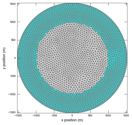
Demonstration of a triangular mesh with the DISV Package to discretize a circular island with a radius of 1500 meters. The model has 2 layers and uses 2778 vertices (NVERT) to delineate 5240 cells per layer (NCPL). General-head boundaries are assigned to model layer 1 for cells outside of a 1025 m radius circle. Recharge is applied to the top of the model.
Initial setup
Import dependencies, define the example name and workspace, and read settings from environment variables.
[1]:
from pathlib import Path

import flopy
import flopy.utils.cvfdutil
import git
import matplotlib.pyplot as plt
import numpy as np
import pooch
from flopy.plot.styles import styles
from flopy.utils.geometry import get_polygon_area
from flopy.utils.gridintersect import GridIntersect
from modflow_devtools.misc import get_env, timed
from shapely.geometry import Polygon

# Example name and workspace paths. If this example is running
# in the git repository, use the folder structure described in
# the README. Otherwise just use the current working directory.
sim_name = "ex-gwf-disvmesh"
try:
    root = Path(git.Repo(".", search_parent_directories=True).working_dir)
except:
    root = None
workspace = root / "examples" if root else Path.cwd()
figs_path = root / "figures" if root else Path.cwd()
data_path = root / "data" / sim_name if root else Path.cwd()

# Settings from environment variables
write = get_env("WRITE", True)
run = get_env("RUN", True)
plot = get_env("PLOT", True)
plot_show = get_env("PLOT_SHOW", True)
plot_save = get_env("PLOT_SAVE", True)
Define parameters
Define model units, parameters and other settings.
[2]:
# Model units
length_units = "meters"
time_units = "days"

# Model parameters
nper = 1  # Number of periods
nlay = 2  # Number of layers
top = 0.0  # Top of the model ($m$)
botm_str = "-20.0, -40.0"  # Layer bottom elevations ($m$)
strt = 0.0  # Starting head ($m$)
icelltype = 0  # Cell conversion type
k11 = 10.0  # Horizontal hydraulic conductivity ($m/d$)
k33 = 0.2  # Vertical hydraulic conductivity ($m/d$)
recharge = 4.0e-3  # Recharge rate ($m/d$)

# Static temporal data used by TDIS file
# Simulation has 1 steady stress period (1 day).
perlen = [1.0]
nstp = [1]
tsmult = [1.0]
tdis_ds = list(zip(perlen, nstp, tsmult))

# Parse strings into lists
botm = [float(value) for value in botm_str.split(",")]


# create the disv grid
def from_argus_export(fname):
    f = open(fname)
    line = f.readline()
    ll = line.split()
    ncells, nverts = ll[0:2]
    ncells = int(ncells)
    nverts = int(nverts)
    verts = np.empty((nverts, 2), dtype=float)

    # read the vertices
    f.readline()
    for ivert in range(nverts):
        line = f.readline()
        ll = line.split()
        c, iv, x, y = ll[0:4]
        verts[ivert, 0] = x
        verts[ivert, 1] = y

    # read the cell information and create iverts
    iverts = []
    for icell in range(ncells):
        line = f.readline()
        ll = line.split()
        ivlist = []
        for ic in ll[2:5]:
            ivlist.append(int(ic) - 1)
        if ivlist[0] != ivlist[-1]:
            ivlist.append(ivlist[0])
        ivlist.reverse()
        iverts.append(ivlist)

    # close file and return spatial reference
    f.close()
    return verts, iverts


# Load argus mesh and get disv grid properties
fname = "argus.exp"
fpath = pooch.retrieve(
    url=f"https://github.com/MODFLOW-ORG/modflow6-examples/raw/master/data/{sim_name}/{fname}",
    fname=fname,
    path=data_path,
    known_hash="md5:072a758ca3d35831acb7e1e27e7b8524",
)
verts, iverts = from_argus_export(fpath)
gridprops = flopy.utils.cvfdutil.get_disv_gridprops(verts, iverts)
cell_areas = []
for i in range(gridprops["ncpl"]):
    x = verts[iverts[i], 0]
    y = verts[iverts[i], 1]
    cell_verts = np.vstack((x, y)).transpose()
    cell_areas.append(get_polygon_area(cell_verts))

# Solver parameters
nouter = 50
ninner = 100
hclose = 1e-9
rclose = 1e-6
Model setup
Define functions to build models, write input files, and run the simulation.
[3]:
def build_models(sim_name):
    sim_ws = workspace / sim_name
    sim = flopy.mf6.MFSimulation(sim_name=sim_name, sim_ws=sim_ws, exe_name="mf6")
    flopy.mf6.ModflowTdis(sim, nper=nper, perioddata=tdis_ds, time_units=time_units)
    flopy.mf6.ModflowIms(
        sim,
        linear_acceleration="bicgstab",
        outer_maximum=nouter,
        outer_dvclose=hclose,
        inner_maximum=ninner,
        inner_dvclose=hclose,
        rcloserecord=f"{rclose} strict",
    )
    gwf = flopy.mf6.ModflowGwf(sim, modelname=sim_name, save_flows=True)
    flopy.mf6.ModflowGwfdisv(
        gwf,
        length_units=length_units,
        nlay=nlay,
        top=top,
        botm=botm,
        **gridprops,
    )
    flopy.mf6.ModflowGwfnpf(
        gwf,
        icelltype=icelltype,
        k=k11,
        k33=k33,
        save_specific_discharge=True,
        xt3doptions=True,
    )
    flopy.mf6.ModflowGwfic(gwf, strt=strt)

    theta = np.arange(0.0, 2 * np.pi, 0.2)
    radius = 1500.0
    x = radius * np.cos(theta)
    y = radius * np.sin(theta)
    outer = [(x, y) for x, y in zip(x, y)]
    radius = 1025.0
    x = radius * np.cos(theta)
    y = radius * np.sin(theta)
    hole = [(x, y) for x, y in zip(x, y)]
    p = Polygon(outer, holes=[hole])
    ix = GridIntersect(gwf.modelgrid)
    result = ix.intersect(p, geo_dataframe=False)
    ghb_cellids = np.array(result["cellids"], dtype=int)

    ghb_spd = []
    ghb_spd += [[0, i, 0.0, k33 * cell_areas[i] / 10.0] for i in ghb_cellids]
    ghb_spd = {0: ghb_spd}
    flopy.mf6.ModflowGwfghb(
        gwf,
        stress_period_data=ghb_spd,
        pname="GHB",
    )

    ncpl = gridprops["ncpl"]
    rchcells = np.array(list(range(ncpl)), dtype=int)
    rchcells[ghb_cellids] = -1
    rch_spd = [(0, rchcells[i], recharge) for i in range(ncpl) if rchcells[i] > 0]
    rch_spd = {0: rch_spd}
    flopy.mf6.ModflowGwfrch(gwf, stress_period_data=rch_spd, pname="RCH")

    head_filerecord = f"{sim_name}.hds"
    budget_filerecord = f"{sim_name}.cbc"
    flopy.mf6.ModflowGwfoc(
        gwf,
        head_filerecord=head_filerecord,
        budget_filerecord=budget_filerecord,
        saverecord=[("HEAD", "ALL"), ("BUDGET", "ALL")],
    )

    return sim


def write_models(sim, silent=True):
    sim.write_simulation(silent=silent)


@timed
def run_models(sim, silent=False):
    success, buff = sim.run_simulation(silent=silent, report=True)
    assert success, buff
Plotting results
Define functions to plot model results.
[4]:
# Figure properties
figure_size = (5, 5)
def plot_grid(idx, sim):
with styles.USGSMap():
sim_ws = workspace / sim_name
gwf = sim.get_model(sim_name)
fig = plt.figure(figsize=figure_size)
fig.tight_layout()
ax = fig.add_subplot(1, 1, 1, aspect="equal")
pmv = flopy.plot.PlotMapView(model=gwf, ax=ax, layer=0)
pmv.plot_grid(linewidth=1)
pmv.plot_bc(name="GHB")
ax.set_xlabel("x position (m)")
ax.set_ylabel("y position (m)")
if plot_show:
plt.show()
if plot_save:
fpth = figs_path / f"{sim_name}-grid.png"
fig.savefig(fpth)
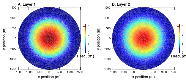
def plot_head(idx, sim):
with styles.USGSMap():
sim_ws = workspace / sim_name
gwf = sim.get_model(sim_name)
fig = plt.figure(figsize=(7.5, 5))
fig.tight_layout()
head = gwf.output.head().get_data()[:, 0, :]
# create MODFLOW 6 cell-by-cell budget object
qx, qy, qz = flopy.utils.postprocessing.get_specific_discharge(
gwf.output.budget().get_data(text="DATA-SPDIS", totim=1.0)[0], gwf
)
ax = fig.add_subplot(1, 2, 1, aspect="equal")
pmv = flopy.plot.PlotMapView(model=gwf, ax=ax, layer=0)
cb = pmv.plot_array(head, cmap="jet", vmin=0.0, vmax=head.max())
pmv.plot_vector(qx, qy, normalize=False, color="0.75")
cbar = plt.colorbar(cb, shrink=0.25)
cbar.ax.set_xlabel(r"Head, ($m$)")
ax.set_xlabel("x position (m)")
ax.set_ylabel("y position (m)")
styles.heading(ax, letter="A", heading="Layer 1")
ax = fig.add_subplot(1, 2, 2, aspect="equal")
pmv = flopy.plot.PlotMapView(model=gwf, ax=ax, layer=1)
cb = pmv.plot_array(head, cmap="jet", vmin=0.0, vmax=head.max())
pmv.plot_vector(qx, qy, normalize=False, color="0.75")
cbar = plt.colorbar(cb, shrink=0.25)
cbar.ax.set_xlabel(r"Head, ($m$)")
ax.set_xlabel("x position (m)")
ax.set_ylabel("y position (m)")
styles.heading(ax, letter="B", heading="Layer 2")
if plot_show:
plt.show()
if plot_save:
fpth = figs_path / f"{sim_name}-head.png"
fig.savefig(fpth)
def plot_results(idx, sim, silent=True):
if idx == 0:
plot_grid(idx, sim)
plot_head(idx, sim)
Running the example
Define and invoke a function to run the example scenario, then plot results.
[5]:
def scenario(idx, silent=True):
    sim = build_models(sim_name)
    if write:
        write_models(sim, silent=silent)
    if run:
        run_models(sim, silent=silent)
    if plot:
        plot_results(idx, sim, silent=silent)


scenario(0)
<flopy.mf6.data.mfstructure.MFDataItemStructure object at 0x7fd50513c2d0>
run_models took 173.70 ms