This page was generated from
ex-gwf-csub-p04.py.
It's also available as a notebook.
One-Dimensional Compaction in a Three-Dimensional Flow Field
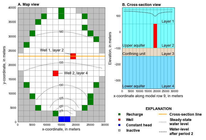
This problem is based on the problem presented in the SUB-WT report (Leake and Galloway, 2007) and represent groundwater development in a hypothetical aquifer that includes some features typical of basin-fill aquifers in an arid or semi-arid environment.
Initial setup
Import dependencies, define the example name and workspace, and read settings from environment variables.
[1]:
from pathlib import Path

import flopy
import git
import matplotlib as mpl
import matplotlib.pyplot as plt
import numpy as np
import pooch
from flopy.plot.styles import styles
from modflow_devtools.misc import get_env, timed

# Example name and workspace paths. If this example is running
# in the git repository, use the folder structure described in
# the README. Otherwise just use the current working directory.
sim_name = "ex-gwf-csub-p04"
try:
    root = Path(git.Repo(".", search_parent_directories=True).working_dir)
except:
    root = None
workspace = root / "examples" if root else Path.cwd()
figs_path = root / "figures" if root else Path.cwd()
data_path = root / "data" / sim_name if root else Path.cwd()

# Settings from environment variables
write = get_env("WRITE", True)
run = get_env("RUN", True)
plot = get_env("PLOT", True)
plot_show = get_env("PLOT_SHOW", True)
plot_save = get_env("PLOT_SAVE", True)
Define parameters
Define model units, parameters and other settings.
[2]:
# Model units
length_units = "meters"
time_units = "days"

# Model parameters
nper = 3  # Number of periods
nlay = 4  # Number of layers
nrow = 20  # Number of rows
ncol = 15  # Number of columns
delr = 2000.0  # Column width ($m$)
delc = 2000.0  # Row width ($m$)
top = 150.0  # Top of the model ($ft$)
botm_str = "50., -100., -150., -350."  # Layer bottom elevations ($m$)
strt = 100.0  # Starting head ($m$)
icelltype_str = "1, 0, 0, 0"  # Cell conversion type
k11_str = "4., 4., 0.01, 4."  # Horizontal hydraulic conductivity ($m/d$)
k33_str = "0.4, 0.4, 0.01, 0.4"  # Vertical hydraulic conductivity ($m/d$)
sy_str = "0.3, 0.3, 0.4, 0.3"  # Specific yield (unitless)
gammaw = 9806.65  # Compressibility of water (Newtons/($m^3$)
beta = 4.6612e-10  # Specific gravity of water (1/$Pa$)
sgm_str = "1.77, 1.77, 1.60, 1.77"  # Specific gravity of moist soils (unitless)
sgs_str = "2.06, 2.05, 1.94, 2.06"  # Specific gravity of saturated soils (unitless)
cg_theta_str = "0.32, 0.32, 0.45, 0.32"  # Coarse-grained material porosity (unitless)
cg_ske_str = "0.005, 0.005, 0.01, 0.005"  # Elastic specific storage ($1/m$)
ib_thick_str = "45., 70., 50., 90."  # Interbed thickness ($m$)
ib_theta = 0.45  # Interbed initial porosity (unitless)
ib_cr = 0.01  # Interbed recompression index (unitless)
ib_cv = 0.25  # Interbed compression index (unitless)
stress_offset = 15.0  # Initial preconsolidation stress offset ($m$)

# Static temporal data used by TDIS file
tdis_ds = (
    (0.0, 1, 1.0),
    (21915.0, 60, 1.0),
    (21915.0, 60, 1.0),
)

# Parse parameter strings into tuples
botm = [float(value) for value in botm_str.split(",")]
icelltype = [int(value) for value in icelltype_str.split(",")]
k11 = [float(value) for value in k11_str.split(",")]
k33 = [float(value) for value in k33_str.split(",")]
sy = [float(value) for value in sy_str.split(",")]
sgm = [float(value) for value in sgm_str.split(",")]
sgs = [float(value) for value in sgs_str.split(",")]
cg_theta = [float(value) for value in cg_theta_str.split(",")]
cg_ske = [float(value) for value in cg_ske_str.split(",")]
ib_thick = [float(value) for value in ib_thick_str.split(",")]

# Load active domain and create idomain array
fname = "idomain.txt"
fpath = pooch.retrieve(
    url=f"https://github.com/MODFLOW-ORG/modflow6-examples/raw/master/data/{sim_name}/{fname}",
    fname=fname,
    path=data_path,
    known_hash="md5:2f05a27b6f71e564c0d3616e3fd00ac8",
)
ib = np.loadtxt(fpath, dtype=int)
idomain = np.tile(ib, (nlay, 1))

# Constant head boundary cells
chd_locs = [(nrow - 1, 7), (nrow - 1, 8)]
c6 = []
for i, j in chd_locs:
    for k in range(nlay):
        c6.append([k, i, j, strt])

# Recharge boundary cells
rch_rate = 5.5e-4
rch6 = []
for i in range(nrow):
    for j in range(ncol):
        if ib[i, j] != 2 or (i, j) in chd_locs:
            continue
        rch6.append([0, i, j, rch_rate])

# Well boundary cells
well_locs = (
    (1, 8, 9),
    (3, 11, 6),
)
well_rates = (
    -72000,
    0.0,
)
wel6 = {}
for idx, q in enumerate(well_rates):
    spd = []
    for k, i, j in well_locs:
        spd.append([k, i, j, q])
    wel6[idx + 1] = spd

# Create interbed package data
icsubno = 0
csub_pakdata = []
boundname_dict = {}
for i in range(nrow):
    for j in range(ncol):
        if ib[i, j] < 1 or (i, j) in chd_locs:
            continue
        for k in range(nlay):
            boundname = f"{k + 1:02d}_{i + 1:02d}_{j + 1:02d}"
            boundname_dict[boundname] = (icsubno,)
            ib_lst = [
                icsubno,
                (k, i, j),
                "nodelay",
                stress_offset,
                ib_thick[k],
                1.0,
                ib_cv,
                ib_cr,
                ib_theta,
                999.0,
                999.0,
                boundname,
            ]
            csub_pakdata.append(ib_lst)
            icsubno += 1

# Solver parameters
nouter = 100
ninner = 300
hclose = 1e-9
rclose = 1e-6
linaccel = "bicgstab"
relax = 0.97
Model setup
Define functions to build models, write input files, and run the simulation.
[3]:
def build_models():
    sim_ws = workspace / sim_name
    sim = flopy.mf6.MFSimulation(sim_name=sim_name, sim_ws=sim_ws, exe_name="mf6")
    flopy.mf6.ModflowTdis(sim, nper=nper, perioddata=tdis_ds, time_units=time_units)
    flopy.mf6.ModflowIms(
        sim,
        outer_maximum=nouter,
        outer_dvclose=hclose,
        linear_acceleration=linaccel,
        inner_maximum=ninner,
        inner_dvclose=hclose,
        relaxation_factor=relax,
        rcloserecord=f"{rclose} strict",
    )
    gwf = flopy.mf6.ModflowGwf(
        sim, modelname=sim_name, save_flows=True, newtonoptions="newton"
    )
    flopy.mf6.ModflowGwfdis(
        gwf,
        length_units=length_units,
        nlay=nlay,
        nrow=nrow,
        ncol=ncol,
        delr=delr,
        delc=delc,
        top=top,
        botm=botm,
        idomain=idomain,
    )
    # gwf obs
    flopy.mf6.ModflowUtlobs(
        gwf,
        digits=10,
        print_input=True,
        continuous={
            "gwf_obs.csv": [
                ("h1l1", "HEAD", (0, 8, 9)),
                ("h1l2", "HEAD", (1, 8, 9)),
                ("h1l3", "HEAD", (2, 8, 9)),
                ("h1l4", "HEAD", (3, 8, 9)),
                ("h2l1", "HEAD", (0, 11, 6)),
                ("h2l2", "HEAD", (1, 11, 6)),
                ("h3l2", "HEAD", (2, 11, 6)),
                ("h4l2", "HEAD", (3, 11, 6)),
            ]
        },
    )

    flopy.mf6.ModflowGwfic(gwf, strt=strt)
    flopy.mf6.ModflowGwfnpf(
        gwf,
        icelltype=icelltype,
        k=k11,
        save_specific_discharge=True,
    )
    flopy.mf6.ModflowGwfsto(
        gwf,
        iconvert=icelltype,
        ss=0.0,
        sy=sy,
        steady_state={0: True},
        transient={1: True},
    )
    csub = flopy.mf6.ModflowGwfcsub(
        gwf,
        print_input=True,
        save_flows=True,
        compression_indices=True,
        update_material_properties=True,
        boundnames=True,
        ninterbeds=len(csub_pakdata),
        sgm=sgm,
        sgs=sgs,
        cg_theta=cg_theta,
        cg_ske_cr=cg_ske,
        beta=beta,
        gammaw=gammaw,
        packagedata=csub_pakdata,
    )
    opth = f"{sim_name}.csub.obs"
    csub_csv = opth + ".csv"
    obs = [
        ("w1l1", "interbed-compaction", boundname_dict["01_09_10"]),
        ("w1l2", "interbed-compaction", boundname_dict["02_09_10"]),
        ("w1l3", "interbed-compaction", boundname_dict["03_09_10"]),
        ("w1l4", "interbed-compaction", boundname_dict["04_09_10"]),
        ("w2l1", "interbed-compaction", boundname_dict["01_12_07"]),
        ("w2l2", "interbed-compaction", boundname_dict["02_12_07"]),
        ("w2l3", "interbed-compaction", boundname_dict["03_12_07"]),
        ("w2l4", "interbed-compaction", boundname_dict["04_12_07"]),
        ("s1l1", "coarse-compaction", (0, 8, 9)),
        ("s1l2", "coarse-compaction", (1, 8, 9)),
        ("s1l3", "coarse-compaction", (2, 8, 9)),
        ("s1l4", "coarse-compaction", (3, 8, 9)),
        ("s2l1", "coarse-compaction", (0, 11, 6)),
        ("s2l2", "coarse-compaction", (1, 11, 6)),
        ("s2l3", "coarse-compaction", (2, 11, 6)),
        ("s2l4", "coarse-compaction", (3, 11, 6)),
        ("c1l1", "compaction-cell", (0, 8, 9)),
        ("c1l2", "compaction-cell", (1, 8, 9)),
        ("c1l3", "compaction-cell", (2, 8, 9)),
        ("c1l4", "compaction-cell", (3, 8, 9)),
        ("c2l1", "compaction-cell", (0, 11, 6)),
        ("c2l2", "compaction-cell", (1, 11, 6)),
        ("c2l3", "compaction-cell", (2, 11, 6)),
        ("c2l4", "compaction-cell", (3, 11, 6)),
        ("w2l4q", "csub-cell", (3, 11, 6)),
        ("gs1", "gstress-cell", (0, 8, 9)),
        ("es1", "estress-cell", (0, 8, 9)),
        ("pc1", "preconstress-cell", (0, 8, 9)),
        ("gs2", "gstress-cell", (1, 8, 9)),
        ("es2", "estress-cell", (1, 8, 9)),
        ("pc2", "preconstress-cell", (1, 8, 9)),
        ("gs3", "gstress-cell", (2, 8, 9)),
        ("es3", "estress-cell", (2, 8, 9)),
        ("pc3", "preconstress-cell", (2, 8, 9)),
        ("gs4", "gstress-cell", (3, 8, 9)),
        ("es4", "estress-cell", (3, 8, 9)),
        ("pc4", "preconstress-cell", (3, 8, 9)),
        ("sk1l2", "ske-cell", (1, 8, 9)),
        ("sk2l4", "ske-cell", (3, 11, 6)),
        ("t1l2", "theta", (1, 8, 9)),
        ("w1qie", "elastic-csub", boundname_dict["02_09_10"]),
        ("w1qii", "inelastic-csub", boundname_dict["02_09_10"]),
        ("w1qaq", "coarse-csub", (1, 8, 9)),
        ("w1qt", "csub-cell", (1, 8, 9)),
        ("w1wc", "wcomp-csub-cell", (1, 8, 9)),
        ("w2qie", "elastic-csub", boundname_dict["04_12_07"]),
        ("w2qii", "inelastic-csub", boundname_dict["04_12_07"]),
        ("w2qaq", "coarse-csub", (3, 11, 6)),
        ("w2qt ", "csub-cell", (3, 11, 6)),
        ("w2wc", "wcomp-csub-cell", (3, 11, 6)),
    ]
    orecarray = {csub_csv: obs}
    csub.obs.initialize(
        filename=opth, digits=10, print_input=True, continuous=orecarray
    )

    flopy.mf6.ModflowGwfchd(gwf, stress_period_data={0: c6})
    flopy.mf6.ModflowGwfrch(gwf, stress_period_data={0: rch6})
    flopy.mf6.ModflowGwfwel(gwf, stress_period_data=wel6)

    head_filerecord = f"{sim_name}.hds"
    budget_filerecord = f"{sim_name}.cbc"
    flopy.mf6.ModflowGwfoc(
        gwf,
        head_filerecord=head_filerecord,
        budget_filerecord=budget_filerecord,
        printrecord=[("BUDGET", "ALL")],
        saverecord=[("BUDGET", "ALL"), ("HEAD", "ALL")],
    )
    return sim


def write_models(sim, silent=True):
    sim.write_simulation(silent=silent)


@timed
def run_models(sim, silent=True):
    success, buff = sim.run_simulation(silent=silent)
    assert success, buff
Plotting results
Define functions to plot model results, starting with a few utilities.
[4]:
# Set figure properties specific to the problem
figure_size = (6.8, 5.5)
arrow_props = {"facecolor": "black", "arrowstyle": "-", "lw": 0.5}
plot_tags = (
"W1L",
"W2L",
"S1L",
"S2L",
"C1L",
"C2L",
)
compaction_heading = ("row 9, column 10", "row 12, column 7")
def get_csub_observations(sim):
name = sim.name
gwf = sim.get_model(sim_name)
csub_obs = gwf.csub.output.obs().data
csub_obs["totim"] /= 365.25
# set initial preconsolidation stress to stress period 1 value
slist = [name for name in csub_obs.dtype.names if "PC" in name]
for tag in slist:
csub_obs[tag][0] = csub_obs[tag][1]
# set initial storativity to stress period 1 value
sk_tags = (
"SK1L2",
"SK2L4",
)
for tag in sk_tags:
if tag in csub_obs.dtype.names:
csub_obs[tag][0] = csub_obs[tag][1]
return csub_obs
def calc_compaction_at_surface(sim):
"""Calculate the compaction at the surface"""
csub_obs = get_csub_observations(sim)
for tag in plot_tags:
for k in (3, 2, 1):
tag0 = f"{tag}{k}"
tag1 = f"{tag}{k + 1}"
csub_obs[tag0] += csub_obs[tag1]
return csub_obs
def plot_compaction_values(ax, sim, tagbase="W1L"):
colors = ["#FFF8DC", "#D2B48C", "#CD853F", "#8B4513"][::-1]
obs = calc_compaction_at_surface(sim)
for k in range(nlay):
fc = colors[k]
tag = f"{tagbase}{k + 1}"
label = f"Layer {k + 1}"
ax.fill_between(obs["totim"], obs[tag], y2=0, color=fc, label=label)
def plot_grid(sim, silent=True):
with styles.USGSMap():
name = sim.name
gwf = sim.get_model(name)
extents = gwf.modelgrid.extent
# read simulated heads
hobj = gwf.output.head()
h0 = hobj.get_data(kstpkper=(0, 0))
h1 = hobj.get_data(kstpkper=(59, 1))
hsxs0 = h0[0, 8, :]
hsxs1 = h1[0, 8, :]
# get delr array
dx = gwf.dis.delr.array
# create x-axis for cross-section
hxloc = np.arange(1000, 2000.0 * 15, 2000.0)
# set cross-section location
y = 2000.0 * 11.5
xsloc = [(extents[0], extents[1]), (y, y)]
# well locations
w1loc = (9.5 * 2000.0, 11.75 * 2000.0)
w2loc = (6.5 * 2000.0, 8.5 * 2000.0)
fig = plt.figure(figsize=(6.8, 5), constrained_layout=True)
gs = mpl.gridspec.GridSpec(7, 10, figure=fig, wspace=100)
plt.axis("off")
ax = fig.add_subplot(gs[:, 0:6])
# ax.set_aspect('equal')
mm = flopy.plot.PlotMapView(model=gwf, ax=ax, extent=extents)
mm.plot_grid(lw=0.5, color="0.5")
mm.plot_bc(ftype="WEL", kper=1, plotAll=True)
mm.plot_bc(ftype="CHD", color="blue")
mm.plot_bc(ftype="RCH", color="green")
mm.plot_inactive(color_noflow="0.75")
mm.ax.plot(xsloc[0], xsloc[1], color="orange", lw=1.5)
# contour steady state heads
cl = mm.contour_array(
h0,
masked_values=[1.0e30],
levels=np.arange(115, 200, 5),
colors="black",
linestyles="dotted",
linewidths=0.75,
)
ax.clabel(cl, fmt="%3i", inline_spacing=0.1)
# well text
styles.add_annotation(
ax=ax,
text="Well 1, layer 2",
bold=False,
italic=False,
xy=w1loc,
xytext=(w1loc[0] - 3200, w1loc[1] + 1500),
ha="right",
va="center",
zorder=100,
arrowprops=arrow_props,
)
styles.add_annotation(
ax=ax,
text="Well 2, layer 4",
bold=False,
italic=False,
xy=w2loc,
xytext=(w2loc[0] + 3000, w2loc[1]),
ha="left",
va="center",
zorder=100,
arrowprops=arrow_props,
)
ax.set_ylabel("y-coordinate, in meters")
ax.set_xlabel("x-coordinate, in meters")
styles.heading(ax, letter="A", heading="Map view")
styles.remove_edge_ticks(ax)
ax = fig.add_subplot(gs[0:5, 6:])
mm = flopy.plot.PlotCrossSection(model=gwf, ax=ax, line={"row": 8})
mm.plot_grid(lw=0.5, color="0.5")
# items for legend
mm.ax.plot(
-1000,
-1000,
"s",
ms=5,
color="green",
mec="black",
mew=0.5,
label="Recharge",
)
mm.ax.plot(
-1000, -1000, "s", ms=5, color="red", mec="black", mew=0.5, label="Well"
)
mm.ax.plot(
-1000,
-1000,
"s",
ms=5,
color="blue",
mec="black",
mew=0.5,
label="Constant head",
)
mm.ax.plot(
-1000,
-1000,
"s",
ms=5,
color="0.75",
mec="black",
mew=0.5,
label="Inactive",
)
mm.ax.plot(
[-1000, -1001],
[-1000, -1000],
color="orange",
lw=1.5,
label="Cross-section line",
)
# aquifer coloring
ax.fill_between([0, dx.sum()], y1=150, y2=-100, color="cyan", alpha=0.5)
ax.fill_between([0, dx.sum()], y1=-100, y2=-150, color="#D2B48C", alpha=0.5)
ax.fill_between([0, dx.sum()], y1=-150, y2=-350, color="#00BFFF", alpha=0.5)
# well coloring
ax.fill_between(
[dx.cumsum()[8], dx.cumsum()[9]], y1=50, y2=-100, color="red", lw=0
)
# labels
styles.add_text(
ax=ax,
transform=False,
bold=False,
italic=False,
x=300,
y=-97,
text="Upper aquifer",
va="bottom",
ha="left",
fontsize=9,
)
styles.add_text(
ax=ax,
transform=False,
bold=False,
italic=False,
x=300,
y=-147,
text="Confining unit",
va="bottom",
ha="left",
fontsize=9,
)
styles.add_text(
ax=ax,
transform=False,
bold=False,
italic=False,
x=300,
y=-347,
text="Lower aquifer",
va="bottom",
ha="left",
fontsize=9,
)
styles.add_text(
ax=ax,
transform=False,
bold=False,
italic=False,
x=29850,
y=53,
text="Layer 1",
va="bottom",
ha="right",
fontsize=9,
)
styles.add_text(
ax=ax,
transform=False,
bold=False,
italic=False,
x=29850,
y=-97,
text="Layer 2",
va="bottom",
ha="right",
fontsize=9,
)
styles.add_text(
ax=ax,
transform=False,
bold=False,
italic=False,
x=29850,
y=-147,
text="Layer 3",
va="bottom",
ha="right",
fontsize=9,
)
styles.add_text(
ax=ax,
transform=False,
bold=False,
italic=False,
x=29850,
y=-347,
text="Layer 4",
va="bottom",
ha="right",
fontsize=9,
)
ax.plot(
hxloc,
hsxs0,
lw=0.75,
color="black",
ls="dotted",
label="Steady-state\nwater level",
)
ax.plot(
hxloc,
hsxs1,
lw=0.75,
color="black",
ls="dashed",
label="Water-level\nafter period 2",
)
ax.set_ylabel("Elevation, in meters")
ax.set_xlabel("x-coordinate along model row 9, in meters")
styles.graph_legend(
mm.ax,
ncol=2,
bbox_to_anchor=(0.7, -0.6),
borderaxespad=0,
frameon=False,
loc="lower center",
)
styles.heading(ax, letter="B", heading="Cross-section view")
styles.remove_edge_ticks(ax)
if plot_show:
plt.show()
if plot_save:
fpth = figs_path / f"{sim_name}-grid.png"
if not silent:
print(f"saving...'{fpth}'")
fig.savefig(fpth)
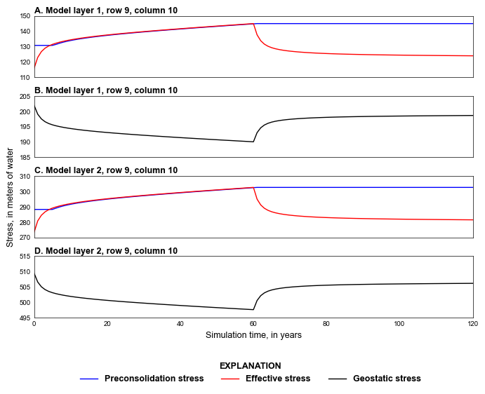
def plot_stresses(sim, silent=True):
with styles.USGSPlot() as fs:
name = sim.name
cd = get_csub_observations(sim)
tmax = cd["totim"][-1]
fig, axes = plt.subplots(
ncols=1, nrows=4, figsize=figure_size, sharex=True, constrained_layout=True
)
idx = 0
ax = axes[idx]
ax.set_xlim(0, tmax)
ax.set_ylim(110, 150)
ax.plot(
cd["totim"], cd["PC1"], color="blue", lw=1, label="Preconsolidation stress"
)
ax.plot(cd["totim"], cd["ES1"], color="red", lw=1, label="Effective stress")
styles.heading(ax, letter="A", heading="Model layer 1, row 9, column 10")
styles.remove_edge_ticks(ax)
idx += 1
ax = axes[idx]
ax.set_ylim(185, 205)
ax.plot(cd["totim"], cd["GS1"], color="black", lw=1)
styles.heading(ax, letter="B", heading="Model layer 1, row 9, column 10")
styles.remove_edge_ticks(ax)
idx += 1
ax = axes[idx]
ax.set_ylim(270, 310)
ax.plot(cd["totim"], cd["PC2"], color="blue", lw=1)
ax.plot(cd["totim"], cd["ES2"], color="red", lw=1)
styles.heading(ax, letter="C", heading="Model layer 2, row 9, column 10")
styles.remove_edge_ticks(ax)
idx += 1
ax = axes[idx]
ax.set_ylim(495, 515)
ax.plot(
[-100, -50],
[-100, -100],
color="blue",
lw=1,
label="Preconsolidation stress",
)
ax.plot([-100, -50], [-100, -100], color="red", lw=1, label="Effective stress")
ax.plot(cd["totim"], cd["GS2"], color="black", lw=1, label="Geostatic stress")
styles.graph_legend(ax, ncol=3, bbox_to_anchor=(0.9, -0.6))
styles.heading(ax, letter="D", heading="Model layer 2, row 9, column 10")
styles.remove_edge_ticks(ax)
ax.set_xlabel("Simulation time, in years")
ax.set_ylabel(" ")
ax = fig.add_subplot(111, frame_on=False, xticks=[], yticks=[])
ax.set_ylabel("Stress, in meters of water")
if plot_show:
plt.show()
if plot_save:
fpth = figs_path / f"{name}-01.png"
if not silent:
print(f"saving...'{fpth}'")
fig.savefig(fpth)
def plot_compaction(sim, silent=True):
with styles.USGSPlot():
name = sim.name
fig, axes = plt.subplots(
ncols=2, nrows=3, figsize=figure_size, sharex=True, constrained_layout=True
)
axes = axes.flatten()
idx = 0
ax = axes[idx]
ax.set_xlim(0, 120)
ax.set_ylim(0, 1)
plot_compaction_values(ax, sim, tagbase=plot_tags[idx])
ht = f"Interbed compaction\n{compaction_heading[0]}"
styles.heading(ax, letter="A", heading=ht)
styles.remove_edge_ticks(ax)
idx += 1
ax = axes[idx]
ax.set_ylim(0, 1)
plot_compaction_values(ax, sim, tagbase=plot_tags[idx])
ht = f"Interbed compaction\n{compaction_heading[1]}"
styles.heading(ax, letter="B", heading=ht)
styles.remove_edge_ticks(ax)
idx += 1
ax = axes[idx]
ax.set_ylim(0, 1)
plot_compaction_values(ax, sim, tagbase=plot_tags[idx])
ht = f"Coarse-grained compaction\n{compaction_heading[0]}"
styles.heading(ax, letter="C", heading=ht)
styles.remove_edge_ticks(ax)
idx += 1
ax = axes[idx]
ax.set_ylim(0, 1)
plot_compaction_values(ax, sim, tagbase=plot_tags[idx])
ht = f"Coarse-grained compaction\n{compaction_heading[1]}"
styles.heading(ax, letter="D", heading=ht)
styles.remove_edge_ticks(ax)
styles.graph_legend(ax, ncol=2, loc="lower right")
idx += 1
ax = axes[idx]
ax.set_ylim(0, 1)
plot_compaction_values(ax, sim, tagbase=plot_tags[idx])
ht = f"Total compaction\n{compaction_heading[0]}"
styles.heading(ax, letter="E", heading=ht)
styles.remove_edge_ticks(ax)
ax.set_ylabel(" ")
ax.set_xlabel(" ")
idx += 1
ax = axes.flat[idx]
ax.set_ylim(0, 1)
plot_compaction_values(ax, sim, tagbase=plot_tags[idx])
ht = f"Total compaction\n{compaction_heading[1]}"
styles.heading(ax, letter="F", heading=ht)
styles.remove_edge_ticks(ax)
ax = fig.add_subplot(111, frame_on=False, xticks=[], yticks=[])
ax.set_ylabel(
"Downward vertical displacement at the top of the model layer, in meters"
)
ax.set_xlabel("Simulation time, in years")
if plot_show:
plt.show()
if plot_save:
fpth = figs_path / f"{name}-02.png"
if not silent:
print(f"saving...'{fpth}'")
fig.savefig(fpth)
def plot_results(sim, silent=True):
plot_grid(sim, silent=silent)
plot_stresses(sim, silent=silent)
plot_compaction(sim, silent=silent)
Running the example
Define and invoke a function to run the example scenario, then plot results.
[5]:
def scenario(silent=False):
    sim = build_models()
    if write:
        write_models(sim, silent=silent)
    if run:
        run_models(sim, silent=silent)
    if plot:
        plot_results(sim, silent=silent)


scenario()
<flopy.mf6.data.mfstructure.MFDataItemStructure object at 0x7fe4b04e0e10>
writing simulation...
  writing simulation name file...
  writing simulation tdis package...
  writing solution package ims_-1...
  writing model ex-gwf-csub-p04...
    writing model name file...
    writing package dis...
    writing package obs_0...
    writing package ic...
    writing package npf...
    writing package sto...
    writing package csub...
    writing package obs_1...
    writing package chd_0...
INFORMATION: maxbound in ('', 'chd', 'dimensions') changed to 8 based on size of stress_period_data
    writing package rch_0...
INFORMATION: maxbound in ('', 'rch', 'dimensions') changed to 18 based on size of stress_period_data
    writing package wel_0...
INFORMATION: maxbound in ('', 'wel', 'dimensions') changed to 2 based on size of stress_period_data
    writing package oc...
FloPy is using the following executable to run the model: ../../../../../../.local/bin/modflow/mf6
                                   MODFLOW 6
                U.S. GEOLOGICAL SURVEY MODULAR HYDROLOGIC MODEL
                  VERSION 6.8.0.dev0 (preliminary) 02/06/2026
                               ***DEVELOP MODE***

        MODFLOW 6 compiled Feb 15 2026 14:55:26 with GCC version 13.3.0

This software is preliminary or provisional and is subject to
revision. It is being provided to meet the need for timely best
science. The software has not received final approval by the U.S.
Geological Survey (USGS). No warranty, expressed or implied, is made
by the USGS or the U.S. Government as to the functionality of the
software and related material nor shall the fact of release
constitute any such warranty. The software is provided on the
condition that neither the USGS nor the U.S. Government shall be held
liable for any damages resulting from the authorized or unauthorized
use of the software.


 MODFLOW runs in SEQUENTIAL mode

 Run start date and time (yyyy/mm/dd hh:mm:ss): 2026/02/15 14:57:34

 Writing simulation list file: mfsim.lst
 Using Simulation name file: mfsim.nam

    Solving:  Stress period:     1    Time step:     1
    Solving:  Stress period:     2    Time step:     1
    Solving:  Stress period:     2    Time step:     2
    Solving:  Stress period:     2    Time step:     3
    Solving:  Stress period:     2    Time step:     4
    Solving:  Stress period:     2    Time step:     5
    Solving:  Stress period:     2    Time step:     6
    Solving:  Stress period:     2    Time step:     7
    Solving:  Stress period:     2    Time step:     8
    Solving:  Stress period:     2    Time step:     9
    Solving:  Stress period:     2    Time step:    10
    Solving:  Stress period:     2    Time step:    11
    Solving:  Stress period:     2    Time step:    12
    Solving:  Stress period:     2    Time step:    13
    Solving:  Stress period:     2    Time step:    14
    Solving:  Stress period:     2    Time step:    15
    Solving:  Stress period:     2    Time step:    16
    Solving:  Stress period:     2    Time step:    17
    Solving:  Stress period:     2    Time step:    18
    Solving:  Stress period:     2    Time step:    19
    Solving:  Stress period:     2    Time step:    20
    Solving:  Stress period:     2    Time step:    21
    Solving:  Stress period:     2    Time step:    22
    Solving:  Stress period:     2    Time step:    23
    Solving:  Stress period:     2    Time step:    24
    Solving:  Stress period:     2    Time step:    25
    Solving:  Stress period:     2    Time step:    26
    Solving:  Stress period:     2    Time step:    27
    Solving:  Stress period:     2    Time step:    28
    Solving:  Stress period:     2    Time step:    29
    Solving:  Stress period:     2    Time step:    30
    Solving:  Stress period:     2    Time step:    31
    Solving:  Stress period:     2    Time step:    32
    Solving:  Stress period:     2    Time step:    33
    Solving:  Stress period:     2    Time step:    34
    Solving:  Stress period:     2    Time step:    35
    Solving:  Stress period:     2    Time step:    36
    Solving:  Stress period:     2    Time step:    37
    Solving:  Stress period:     2    Time step:    38
    Solving:  Stress period:     2    Time step:    39
    Solving:  Stress period:     2    Time step:    40
    Solving:  Stress period:     2    Time step:    41
    Solving:  Stress period:     2    Time step:    42
    Solving:  Stress period:     2    Time step:    43
    Solving:  Stress period:     2    Time step:    44
    Solving:  Stress period:     2    Time step:    45
    Solving:  Stress period:     2    Time step:    46
    Solving:  Stress period:     2    Time step:    47
    Solving:  Stress period:     2    Time step:    48
    Solving:  Stress period:     2    Time step:    49
    Solving:  Stress period:     2    Time step:    50
    Solving:  Stress period:     2    Time step:    51
    Solving:  Stress period:     2    Time step:    52
    Solving:  Stress period:     2    Time step:    53
    Solving:  Stress period:     2    Time step:    54
    Solving:  Stress period:     2    Time step:    55
    Solving:  Stress period:     2    Time step:    56
    Solving:  Stress period:     2    Time step:    57
    Solving:  Stress period:     2    Time step:    58
    Solving:  Stress period:     2    Time step:    59
    Solving:  Stress period:     2    Time step:    60
    Solving:  Stress period:     3    Time step:     1
    Solving:  Stress period:     3    Time step:     2
    Solving:  Stress period:     3    Time step:     3
    Solving:  Stress period:     3    Time step:     4
    Solving:  Stress period:     3    Time step:     5
    Solving:  Stress period:     3    Time step:     6
    Solving:  Stress period:     3    Time step:     7
    Solving:  Stress period:     3    Time step:     8
    Solving:  Stress period:     3    Time step:     9
    Solving:  Stress period:     3    Time step:    10
    Solving:  Stress period:     3    Time step:    11
    Solving:  Stress period:     3    Time step:    12
    Solving:  Stress period:     3    Time step:    13
    Solving:  Stress period:     3    Time step:    14
    Solving:  Stress period:     3    Time step:    15
    Solving:  Stress period:     3    Time step:    16
    Solving:  Stress period:     3    Time step:    17
    Solving:  Stress period:     3    Time step:    18
    Solving:  Stress period:     3    Time step:    19
    Solving:  Stress period:     3    Time step:    20
    Solving:  Stress period:     3    Time step:    21
    Solving:  Stress period:     3    Time step:    22
    Solving:  Stress period:     3    Time step:    23
    Solving:  Stress period:     3    Time step:    24
    Solving:  Stress period:     3    Time step:    25
    Solving:  Stress period:     3    Time step:    26
    Solving:  Stress period:     3    Time step:    27
    Solving:  Stress period:     3    Time step:    28
    Solving:  Stress period:     3    Time step:    29
    Solving:  Stress period:     3    Time step:    30
    Solving:  Stress period:     3    Time step:    31
    Solving:  Stress period:     3    Time step:    32
    Solving:  Stress period:     3    Time step:    33
    Solving:  Stress period:     3    Time step:    34
    Solving:  Stress period:     3    Time step:    35
    Solving:  Stress period:     3    Time step:    36
    Solving:  Stress period:     3    Time step:    37
    Solving:  Stress period:     3    Time step:    38
    Solving:  Stress period:     3    Time step:    39
    Solving:  Stress period:     3    Time step:    40
    Solving:  Stress period:     3    Time step:    41
    Solving:  Stress period:     3    Time step:    42
    Solving:  Stress period:     3    Time step:    43
    Solving:  Stress period:     3    Time step:    44
    Solving:  Stress period:     3    Time step:    45
    Solving:  Stress period:     3    Time step:    46
    Solving:  Stress period:     3    Time step:    47
    Solving:  Stress period:     3    Time step:    48
    Solving:  Stress period:     3    Time step:    49
    Solving:  Stress period:     3    Time step:    50
    Solving:  Stress period:     3    Time step:    51
    Solving:  Stress period:     3    Time step:    52
    Solving:  Stress period:     3    Time step:    53
    Solving:  Stress period:     3    Time step:    54
    Solving:  Stress period:     3    Time step:    55
    Solving:  Stress period:     3    Time step:    56
    Solving:  Stress period:     3    Time step:    57
    Solving:  Stress period:     3    Time step:    58
    Solving:  Stress period:     3    Time step:    59
    Solving:  Stress period:     3    Time step:    60

 Run end date and time (yyyy/mm/dd hh:mm:ss): 2026/02/15 14:57:36
 Elapsed run time:  2.111 Seconds

 Normal termination of simulation.
run_models took 2113.88 ms
/home/runner/work/modflow6-examples/modflow6-examples/modflow6-examples/.pixi/envs/default/lib/python3.13/site-packages/IPython/core/pylabtools.py:170: UserWarning: constrained_layout not applied because axes sizes collapsed to zero.  Try making figure larger or Axes decorations smaller.
  fig.canvas.print_figure(bytes_io, **kw)
saving...'/home/runner/work/modflow6-examples/modflow6-examples/modflow6-examples/figures/ex-gwf-csub-p04-grid.png'
/tmp/ipykernel_9511/1227768118.py:311: UserWarning: constrained_layout not applied because axes sizes collapsed to zero.  Try making figure larger or Axes decorations smaller.
  fig.savefig(fpth)
saving...'/home/runner/work/modflow6-examples/modflow6-examples/modflow6-examples/figures/ex-gwf-csub-p04-01.png'

saving...'/home/runner/work/modflow6-examples/modflow6-examples/modflow6-examples/figures/ex-gwf-csub-p04-02.png'