Flow Diversion
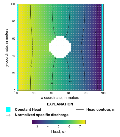
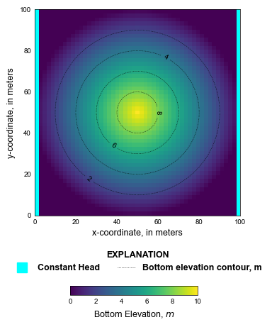
This example simulates unconfined groundwater flow in an aquifer with a high bottom elevation in the center of the aquifer and groundwater flow around a high bottom elevation.
Initial setup
Import dependencies, define the example name and workspace, and read settings from environment variables.
[1]:
from pathlib import Path

import flopy
import git
import matplotlib as mpl
import matplotlib.pyplot as plt
import numpy as np
import pooch
from flopy.plot.styles import styles
from modflow_devtools.misc import get_env, timed

# Example name and workspace paths. If this example is running
# in the git repository, use the folder structure described in
# the README. Otherwise just use the current working directory.
sim_name = "ex-gwf-bump"
try:
    root = Path(git.Repo(".", search_parent_directories=True).working_dir)
except:
    root = None
workspace = root / "examples" if root else Path.cwd()
figs_path = root / "figures" if root else Path.cwd()
data_path = root / "data" / sim_name if root else Path.cwd()

# Settings from environment variables
write = get_env("WRITE", True)
run = get_env("RUN", True)
plot = get_env("PLOT", True)
plot_show = get_env("PLOT_SHOW", True)
plot_save = get_env("PLOT_SAVE", True)
Define parameters
Define model units, parameters and other settings.
[2]:
# Model units
length_units = "meters"
time_units = "days"

# Scenario-specific parameters
parameters = {
    "ex-gwf-bump-p01a": {
        "newton": "newton",
    },
    "ex-gwf-bump-p01b": {
        "rewet": True,
        "wetfct": 1.0,
        "iwetit": 1,
        "ihdwet": 0,
        "wetdry": 2.0,
    },
    "ex-gwf-bump-p01c": {
        "newton": "newton",
        "cylindrical": True,
    },
}

# Model parameters
nper = 1  # Number of periods
nlay = 1  # Number of layers
nrow = 51  # Number of rows
ncol = 51  # Number of columns
xlen = 100.0  # Model length in x-direction ($m$)
ylen = 100.0  # Model length in y-direction ($m$)
top = 25.0  # Top of the model ($m$)
k11 = 1.0  # Horizontal hydraulic conductivity ($m/day$)
H1 = 7.5  # Constant head in column 1 and starting head ($m$)
H2 = 2.5  # Constant head in column 51 ($m$)

# Time discretization
tdis_ds = ((1.0, 1, 1.0),)

# Calculate delr, delc, extents, and shape3d
delr = xlen / float(ncol)
delc = ylen / float(nrow)
extents = (0, xlen, 0, ylen)
shape3d = (nlay, nrow, ncol)

# Load the bottom
fname = "bottom.txt"
fpath = pooch.retrieve(
    url=f"https://github.com/MODFLOW-ORG/modflow6-examples/raw/master/data/{sim_name}/{fname}",
    fname=fname,
    path=data_path,
    known_hash="md5:9287f9e214147d95e6ed159732079a0b",
)
botm = np.loadtxt(fpath).reshape(shape3d)

# Create a cylinder
cylinder = botm.copy()
cylinder[cylinder < 7.5] = 0.0
cylinder[cylinder >= 7.5] = 20.0

# Constant head boundary conditions
chd_spd = [[0, i, 0, H1] for i in range(nrow)]
chd_spd += [[0, i, ncol - 1, H2] for i in range(nrow)]

# Solver parameters
nouter = 500
ninner = 500
hclose = 1e-9
rclose = 1e-6
Model setup
Define functions to build models, write input files, and run the simulation.
[3]:
def build_models(
    name,
    newton=False,
    rewet=False,
    cylindrical=False,
    wetfct=None,
    iwetit=None,
    ihdwet=None,
    wetdry=None,
):
    sim_ws = workspace / name
    sim = flopy.mf6.MFSimulation(sim_name=sim_name, sim_ws=sim_ws, exe_name="mf6")
    flopy.mf6.ModflowTdis(sim, nper=nper, perioddata=tdis_ds, time_units=time_units)
    if newton:
        linear_acceleration = "bicgstab"
        newtonoptions = "newton under_relaxation"
    else:
        linear_acceleration = "cg"
        newtonoptions = None

    flopy.mf6.ModflowIms(
        sim,
        print_option="ALL",
        linear_acceleration=linear_acceleration,
        outer_maximum=nouter,
        outer_dvclose=hclose,
        inner_maximum=ninner,
        inner_dvclose=hclose,
        rcloserecord=rclose,
    )
    gwf = flopy.mf6.ModflowGwf(
        sim,
        modelname=sim_name,
        newtonoptions=newtonoptions,
        save_flows=True,
    )
    if cylindrical:
        bot = cylinder
    else:
        bot = botm
    flopy.mf6.ModflowGwfdis(
        gwf,
        length_units=length_units,
        nlay=nlay,
        nrow=nrow,
        ncol=ncol,
        delr=delr,
        delc=delc,
        top=top,
        botm=bot,
    )
    if rewet:
        rewet_record = ["wetfct", wetfct, "iwetit", iwetit, "ihdwet", ihdwet]
    else:
        rewet_record = None
    flopy.mf6.ModflowGwfnpf(
        gwf,
        rewet_record=rewet_record,
        icelltype=1,
        k=k11,
        wetdry=wetdry,
        save_specific_discharge=True,
    )
    flopy.mf6.ModflowGwfic(gwf, strt=H1)
    flopy.mf6.ModflowGwfchd(gwf, stress_period_data=chd_spd)

    head_filerecord = f"{sim_name}.hds"
    budget_filerecord = f"{sim_name}.cbc"
    flopy.mf6.ModflowGwfoc(
        gwf,
        head_filerecord=head_filerecord,
        budget_filerecord=budget_filerecord,
        saverecord=[("HEAD", "ALL"), ("BUDGET", "ALL")],
    )
    return sim


def write_models(sim, silent=True):
    sim.write_simulation(silent=silent)


@timed
def run_models(sim, silent=True):
    success, buff = sim.run_simulation(silent=silent)
    assert success, buff
Plotting results
Define functions to plot model results.
[4]:
# Figure properties, plotting ranges and contour levels
figure_size = (4, 5.33)
masked_values = (1e30, -1e30)
vmin, vmax = H2, H1
bmin, bmax = 0, 10
vlevels = np.arange(vmin + 0.5, vmax, 1)
blevels = np.arange(bmin + 2, bmax, 2)
bcolor = "black"
vcolor = "black"


def create_figure():
    fig = plt.figure(figsize=figure_size, constrained_layout=False)
    gs = mpl.gridspec.GridSpec(ncols=10, nrows=7, figure=fig, wspace=5)
    plt.axis("off")

    # create axes
    ax1 = fig.add_subplot(gs[:5, :])
    ax2 = fig.add_subplot(gs[5:, :])

    # set limits for map figure
    ax1.set_xlim(extents[:2])
    ax1.set_ylim(extents[2:])
    ax1.set_aspect("equal")

    # set limits for legend area
    ax2.set_xlim(0, 1)
    ax2.set_ylim(0, 1)

    # get rid of ticks and spines for legend area
    ax2.axis("off")
    ax2.set_xticks([])
    ax2.set_yticks([])
    ax2.spines["top"].set_color("none")
    ax2.spines["bottom"].set_color("none")
    ax2.spines["left"].set_color("none")
    ax2.spines["right"].set_color("none")
    ax2.patch.set_alpha(0.0)

    axes = [ax1, ax2]

    return fig, axes


def plot_grid(gwf, silent=True):
    with styles.USGSMap() as fs:
        bot = gwf.dis.botm.array
        fig, axes = create_figure()
        ax = axes[0]
        mm = flopy.plot.PlotMapView(gwf, ax=ax, extent=extents)
        bot_coll = mm.plot_array(bot, vmin=bmin, vmax=bmax)
        mm.plot_bc("CHD", color="cyan")
        cv = mm.contour_array(
            bot, levels=blevels, linewidths=0.5, linestyles=":", colors=bcolor
        )
        plt.clabel(cv, fmt="%1.0f")
        ax.set_xlabel("x-coordinate, in meters")
        ax.set_ylabel("y-coordinate, in meters")
        styles.remove_edge_ticks(ax)

        # legend
        ax = axes[1]
        ax.plot(
            -10000,
            -10000,
            lw=0,
            marker="s",
            ms=10,
            mfc="cyan",
            mec="cyan",
            label="Constant Head",
        )
        ax.plot(
            -10000,
            -10000,
            lw=0.5,
            ls=":",
            color=bcolor,
            label="Bottom elevation contour, m",
        )
        styles.graph_legend(ax, loc="center", ncol=2)

        cax = plt.axes([0.275, 0.125, 0.45, 0.025])
        cbar = plt.colorbar(bot_coll, shrink=0.8, orientation="horizontal", cax=cax)
        cbar.ax.tick_params(size=0)
        cbar.ax.set_xlabel(r"Bottom Elevation, $m$")

        if plot_show:
            plt.show()
        if plot_save:
            fpth = figs_path / f"{sim_name}-grid.png"
            fig.savefig(fpth)


def plot_results(idx, sim, silent=True):
    with styles.USGSMap():
        gwf = sim.get_model(sim_name)
        bot = gwf.dis.botm.array

        if idx == 0:
            plot_grid(gwf, silent=silent)

        # create MODFLOW 6 head object
        hobj = gwf.output.head()

        # create MODFLOW 6 cell-by-cell budget object
        cobj = gwf.output.budget()

        # extract heads and specific discharge
        head = hobj.get_data(totim=1.0)
        imask = (head > -1e30) & (head <= bot)
        head[imask] = -1e30  # botm[imask]
        qx, qy, qz = flopy.utils.postprocessing.get_specific_discharge(
            cobj.get_data(text="DATA-SPDIS", totim=1.0)[0], gwf
        )

        # Create figure for simulation
        fig, axes = create_figure()

        ax = axes[0]
        mm = flopy.plot.PlotMapView(gwf, ax=ax, extent=extents)
        if bot.max() < 20:
            cv = mm.contour_array(
                bot,
                levels=blevels,
                linewidths=0.5,
                linestyles=":",
                colors=bcolor,
                zorder=9,
            )
            plt.clabel(cv, fmt="%1.0f", zorder=9)
        h_coll = mm.plot_array(
            head, vmin=vmin, vmax=vmax, masked_values=masked_values, zorder=10
        )
        cv = mm.contour_array(
            head,
            masked_values=masked_values,
            levels=vlevels,
            linewidths=0.5,
            linestyles="-",
            colors=vcolor,
            zorder=10,
        )
        plt.clabel(cv, fmt="%1.0f", zorder=10)
        mm.plot_bc("CHD", color="cyan", zorder=11)
        mm.plot_vector(qx, qy, normalize=True, color="0.75", zorder=11)
        ax.set_xlabel("x-coordinate, in meters")
        ax.set_ylabel("y-coordinate, in meters")
        styles.remove_edge_ticks(ax)

        # create legend
        ax = axes[-1]
        ax.plot(
            -10000,
            -10000,
            lw=0,
            marker="s",
            ms=10,
            mfc="cyan",
            mec="cyan",
            label="Constant Head",
        )
        ax.plot(
            -10000,
            -10000,
            lw=0,
            marker="$\u2192$",
            ms=10,
            mfc="0.75",
            mec="0.75",
            label="Normalized specific discharge",
        )
        if bot.max() < 20:
            ax.plot(
                -10000,
                -10000,
                lw=0.5,
                ls=":",
                color=bcolor,
                label="Bottom elevation contour, m",
            )
        ax.plot(-10000, -10000, lw=0.5, ls="-", color=vcolor, label="Head contour, m")
        styles.graph_legend(ax, loc="center", ncol=2)

        cax = plt.axes([0.275, 0.125, 0.45, 0.025])
        cbar = plt.colorbar(h_coll, shrink=0.8, orientation="horizontal", cax=cax)
        cbar.ax.tick_params(size=0)
        cbar.ax.set_xlabel(r"Head, $m$", fontsize=9)

        if plot_show:
            plt.show()
        if plot_save:
            fig.savefig(figs_path / f"{sim_name}-{idx + 1:02d}.png")
Running the example
Define a function to run the example scenarios and plot results.
[5]:
def scenario(idx, silent=True):
    key = list(parameters.keys())[idx]
    params = parameters[key].copy()
    sim = build_models(key, **params)
    if write:
        write_models(sim, silent=silent)
    if run:
        run_models(sim, silent=silent)
    if plot:
        plot_results(idx, sim, silent=silent)
Run the flow diversion model with Newton-Raphson and plot simulated heads.
[6]:
scenario(0, silent=False)
writing simulation...
  writing simulation name file...
  writing simulation tdis package...
  writing solution package ims_-1...
  writing model ex-gwf-bump...
    writing model name file...
    writing package dis...
    writing package npf...
    writing package ic...
    writing package chd_0...
INFORMATION: maxbound in ('', 'chd', 'dimensions') changed to 102 based on size of stress_period_data
    writing package oc...
FloPy is using the following executable to run the model: ../../../../../../.local/bin/modflow/mf6
                                   MODFLOW 6
                U.S. GEOLOGICAL SURVEY MODULAR HYDROLOGIC MODEL
                  VERSION 6.8.0.dev0 (preliminary) 02/06/2026
                               ***DEVELOP MODE***

        MODFLOW 6 compiled Feb 15 2026 14:55:26 with GCC version 13.3.0

This software is preliminary or provisional and is subject to
revision. It is being provided to meet the need for timely best
science. The software has not received final approval by the U.S.
Geological Survey (USGS). No warranty, expressed or implied, is made
by the USGS or the U.S. Government as to the functionality of the
software and related material nor shall the fact of release
constitute any such warranty. The software is provided on the
condition that neither the USGS nor the U.S. Government shall be held
liable for any damages resulting from the authorized or unauthorized
use of the software.


 MODFLOW runs in SEQUENTIAL mode

 Run start date and time (yyyy/mm/dd hh:mm:ss): 2026/02/15 14:56:15

 Writing simulation list file: mfsim.lst
 Using Simulation name file: mfsim.nam

    Solving:  Stress period:     1    Time step:     1
 Run end date and time (yyyy/mm/dd hh:mm:ss): 2026/02/15 14:56:16
 Elapsed run time:  0.480 Seconds

 Normal termination of simulation.
run_models took 484.02 ms
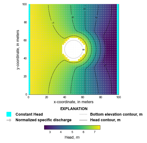
Run the flow diversion model with rewetting and plot simulated heads.
[7]:
scenario(1, silent=False)
writing simulation...
  writing simulation name file...
  writing simulation tdis package...
  writing solution package ims_-1...
  writing model ex-gwf-bump...
    writing model name file...
    writing package dis...
    writing package npf...
    writing package ic...
    writing package chd_0...
INFORMATION: maxbound in ('', 'chd', 'dimensions') changed to 102 based on size of stress_period_data
    writing package oc...
FloPy is using the following executable to run the model: ../../../../../../.local/bin/modflow/mf6
                                   MODFLOW 6
                U.S. GEOLOGICAL SURVEY MODULAR HYDROLOGIC MODEL
                  VERSION 6.8.0.dev0 (preliminary) 02/06/2026
                               ***DEVELOP MODE***

        MODFLOW 6 compiled Feb 15 2026 14:55:26 with GCC version 13.3.0

This software is preliminary or provisional and is subject to
revision. It is being provided to meet the need for timely best
science. The software has not received final approval by the U.S.
Geological Survey (USGS). No warranty, expressed or implied, is made
by the USGS or the U.S. Government as to the functionality of the
software and related material nor shall the fact of release
constitute any such warranty. The software is provided on the
condition that neither the USGS nor the U.S. Government shall be held
liable for any damages resulting from the authorized or unauthorized
use of the software.


 MODFLOW runs in SEQUENTIAL mode

 Run start date and time (yyyy/mm/dd hh:mm:ss): 2026/02/15 14:56:17

 Writing simulation list file: mfsim.lst
 Using Simulation name file: mfsim.nam

    Solving:  Stress period:     1    Time step:     1

 Run end date and time (yyyy/mm/dd hh:mm:ss): 2026/02/15 14:56:17
 Elapsed run time:  0.104 Seconds

 Normal termination of simulation.
run_models took 107.56 ms
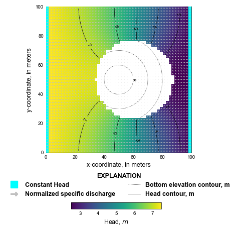
Run the flow diversion model with Newton-Raphson and cylindrical topography and plot simulated heads.
[8]:
scenario(2, silent=False)
writing simulation...
  writing simulation name file...
  writing simulation tdis package...
  writing solution package ims_-1...
  writing model ex-gwf-bump...
    writing model name file...
    writing package dis...
    writing package npf...
    writing package ic...
    writing package chd_0...
INFORMATION: maxbound in ('', 'chd', 'dimensions') changed to 102 based on size of stress_period_data
    writing package oc...
FloPy is using the following executable to run the model: ../../../../../../.local/bin/modflow/mf6
                                   MODFLOW 6
                U.S. GEOLOGICAL SURVEY MODULAR HYDROLOGIC MODEL
                  VERSION 6.8.0.dev0 (preliminary) 02/06/2026
                               ***DEVELOP MODE***

        MODFLOW 6 compiled Feb 15 2026 14:55:26 with GCC version 13.3.0

This software is preliminary or provisional and is subject to
revision. It is being provided to meet the need for timely best
science. The software has not received final approval by the U.S.
Geological Survey (USGS). No warranty, expressed or implied, is made
by the USGS or the U.S. Government as to the functionality of the
software and related material nor shall the fact of release
constitute any such warranty. The software is provided on the
condition that neither the USGS nor the U.S. Government shall be held
liable for any damages resulting from the authorized or unauthorized
use of the software.


 MODFLOW runs in SEQUENTIAL mode

 Run start date and time (yyyy/mm/dd hh:mm:ss): 2026/02/15 14:56:17

 Writing simulation list file: mfsim.lst
 Using Simulation name file: mfsim.nam

    Solving:  Stress period:     1    Time step:     1

 Run end date and time (yyyy/mm/dd hh:mm:ss): 2026/02/15 14:56:17
 Elapsed run time:  0.069 Seconds

 Normal termination of simulation.
run_models took 72.82 ms