This page was generated from
ex-gwf-bcf2ss.py.
It's also available as a notebook.
BCF2SS Model
This problem is described in McDonald and Harbaugh (1988) and duplicated in Harbaugh and McDonald (1996). This problem is also is distributed with MODFLOW-2005 (Harbaugh, 2005) and MODFLOW 6 (Langevin and others, 2017).
Two scenarios are included, first solved with the standard method, then with the Newton-Raphson formulation.
Initial setup
Initial setup
Import dependencies, define the example name and workspace, and read settings from environment variables.
[1]:
from pathlib import Path

import flopy
import git
import matplotlib as mpl
import matplotlib.pyplot as plt
import numpy as np
import pooch
from flopy.plot.styles import styles
from modflow_devtools.misc import get_env, timed

# Example name and workspace paths. If this example is running
# in the git repository, use the folder structure described in
# the README. Otherwise just use the current working directory.
sim_name = "ex-gwf-bcf2ss"
try:
    root = Path(git.Repo(".", search_parent_directories=True).working_dir)
except:
    root = None
workspace = root / "examples" if root else Path.cwd()
figs_path = root / "figures" if root else Path.cwd()
data_path = root / "data" / sim_name if root else Path.cwd()

# Settings from environment variables
write = get_env("WRITE", True)
run = get_env("RUN", True)
plot = get_env("PLOT", True)
plot_show = get_env("PLOT_SHOW", True)
plot_save = get_env("PLOT_SAVE", True)
Define parameters
Define model units, parameters and other settings.
[2]:
# Model units
length_units = "feet"
time_units = "days"
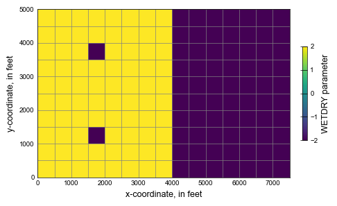
# Load the wetdry array for layer 1
fname = "wetdry01.txt"
fpath = pooch.retrieve(
url=f"https://github.com/MODFLOW-ORG/modflow6-examples/raw/master/data/{sim_name}/{fname}",
fname=fname,
path=data_path,
known_hash="md5:3a4b357b7d2cd5175a205f3347ab973d",
)
wetdry_layer0 = np.loadtxt(fpath)
# Scenario-specific parameters
parameters = {
"ex-gwf-bcf2ss-p01a": {
"rewet": True,
"wetfct": 1.0,
"iwetit": 1,
"ihdwet": 0,
"linear_acceleration": "cg",
"newton": None,
},
"ex-gwf-bcf2ss-p02a": {
"rewet": False,
"wetfct": None,
"iwetit": None,
"ihdwet": None,
"linear_acceleration": "bicgstab",
"newton": "NEWTON",
},
}
# Model parameters
nper = 2 # Number of periods
nlay = 2 # Number of layers
nrow = 10 # Number of rows
ncol = 15 # Number of columns
delr = 500.0 # Column width ($ft$)
delc = 500.0 # Row width ($ft$)
top = 150.0 # Top of the model ($ft$)
botm_str = "50.0, -50." # Layer bottom elevations ($ft$)
icelltype_str = "1, 0" # Cell conversion type
k11_str = "10.0, 5.0" # Horizontal hydraulic conductivity ($ft/d$)
k33 = 0.1 # Vertical hydraulic conductivity ($ft/d$)
strt = 0.0 # Starting head ($ft$)
recharge = 0.004 # Recharge rate ($ft/d$)
# Time discretization
tdis_ds = (
(1.0, 1.0, 1),
(1.0, 1.0, 1),
)
# Parse parameter strings into tuples
botm = [float(value) for value in botm_str.split(",")]
icelltype = [int(value) for value in icelltype_str.split(",")]
k11 = [float(value) for value in k11_str.split(",")]
# Well boundary conditions
wel_spd = {
1: [
[1, 2, 3, -35000.0],
[1, 7, 3, -35000.0],
]
}
# River boundary conditions
riv_spd = {0: [[1, i, 14, 0.0, 10000.0, -5] for i in range(nrow)]}
# Solver parameters
nouter = 500
ninner = 100
hclose = 1e-6
rclose = 1e-3
relax = 0.97
Model setup
Define functions to build models, write input files, and run the simulation.
[3]:
def build_models(name, rewet, wetfct, iwetit, ihdwet, linear_acceleration, newton):
    sim_ws = workspace / name
    sim = flopy.mf6.MFSimulation(sim_name=sim_name, sim_ws=sim_ws, exe_name="mf6")
    flopy.mf6.ModflowTdis(sim, nper=nper, perioddata=tdis_ds, time_units=time_units)
    flopy.mf6.ModflowIms(
        sim,
        linear_acceleration=linear_acceleration,
        outer_maximum=nouter,
        outer_dvclose=hclose,
        inner_maximum=ninner,
        inner_dvclose=hclose,
        rcloserecord=f"{rclose} strict",
        relaxation_factor=relax,
    )
    gwf = flopy.mf6.ModflowGwf(
        sim, modelname=sim_name, save_flows=True, newtonoptions=newton
    )
    flopy.mf6.ModflowGwfdis(
        gwf,
        length_units=length_units,
        nlay=nlay,
        nrow=nrow,
        ncol=ncol,
        delr=delr,
        delc=delc,
        top=top,
        botm=botm,
    )
    if rewet:
        rewet_record = ["wetfct", wetfct, "iwetit", iwetit, "ihdwet", ihdwet]
        wetdry = [wetdry_layer0, 0]
    else:
        rewet_record = None
        wetdry = None

    flopy.mf6.ModflowGwfnpf(
        gwf,
        rewet_record=rewet_record,
        wetdry=wetdry,
        icelltype=icelltype,
        k=k11,
        k33=k33,
        save_specific_discharge=True,
    )
    flopy.mf6.ModflowGwfic(gwf, strt=strt)
    flopy.mf6.ModflowGwfriv(gwf, stress_period_data=riv_spd)
    flopy.mf6.ModflowGwfwel(gwf, stress_period_data=wel_spd)
    flopy.mf6.ModflowGwfrcha(gwf, recharge=recharge)
    head_filerecord = f"{sim_name}.hds"
    budget_filerecord = f"{sim_name}.cbc"
    flopy.mf6.ModflowGwfoc(
        gwf,
        head_filerecord=head_filerecord,
        budget_filerecord=budget_filerecord,
        saverecord=[("HEAD", "ALL"), ("BUDGET", "ALL")],
    )
    return sim


def write_models(sim, silent=True):
    sim.write_simulation(silent=silent)


@timed
def run_models(sim, silent=True):
    success, buff = sim.run_simulation(silent=silent)
    assert success, buff
Plotting results
Define functions to plot model results.
[4]:
# Figure properties
figure_size = (6, 6)
def plot_simulated_results(num, gwf, ho, co, silent=True):
with styles.USGSMap():
botm_arr = gwf.dis.botm.array
fig = plt.figure(figsize=(6.8, 6), constrained_layout=False)
gs = mpl.gridspec.GridSpec(ncols=10, nrows=7, figure=fig, wspace=5)
plt.axis("off")
ax1 = fig.add_subplot(gs[:3, :5])
ax2 = fig.add_subplot(gs[:3, 5:], sharey=ax1)
ax3 = fig.add_subplot(gs[3:6, :5], sharex=ax1)
ax4 = fig.add_subplot(gs[3:6, 5:], sharex=ax1, sharey=ax1)
ax5 = fig.add_subplot(gs[6, :])
axes = [ax1, ax2, ax3, ax4, ax5]
labels = ("A", "B", "C", "D")
aquifer = ("Upper aquifer", "Lower aquifer")
cond = ("natural conditions", "pumping conditions")
vmin, vmax = -10, 140
masked_values = [1e30, -1e30]
levels = [np.arange(0, 130, 10), (10, 20, 30, 40, 50, 55, 60)]
plot_number = 0
for idx, totim in enumerate((1, 2)):
head = ho.get_data(totim=totim)
head[head < botm_arr] = -1e30
qx, qy, qz = flopy.utils.postprocessing.get_specific_discharge(
co.get_data(text="DATA-SPDIS", kstpkper=(0, totim - 1))[0], gwf
)
for k in range(nlay):
ax = axes[plot_number]
ax.set_aspect("equal")
mm = flopy.plot.PlotMapView(model=gwf, ax=ax, layer=k)
mm.plot_grid(lw=0.5, color="0.5")
cm = mm.plot_array(
head, masked_values=masked_values, vmin=vmin, vmax=vmax
)
mm.plot_bc(ftype="WEL", kper=totim - 1)
mm.plot_bc(ftype="RIV", color="green", kper=0)
mm.plot_vector(qx, qy, normalize=True, color="0.75")
cn = mm.contour_array(
head,
masked_values=masked_values,
levels=levels[idx],
colors="black",
linewidths=0.5,
)
plt.clabel(cn, fmt="%3.0f")
heading = f"{aquifer[k]} under\n{cond[totim - 1]}"
styles.heading(ax, letter=labels[plot_number], heading=heading)
styles.remove_edge_ticks(ax)
plot_number += 1
# set axis labels
ax1.set_ylabel("y-coordinate, in feet")
ax3.set_ylabel("y-coordinate, in feet")
ax3.set_xlabel("x-coordinate, in feet")
ax4.set_xlabel("x-coordinate, in feet")
# legend
ax = axes[-1]
ax.set_ylim(1, 0)
ax.set_xlim(-5, 5)
ax.set_xticks([])
ax.set_yticks([])
ax.spines["top"].set_color("none")
ax.spines["bottom"].set_color("none")
ax.spines["left"].set_color("none")
ax.spines["right"].set_color("none")
ax.patch.set_alpha(0.0)
# items for legend
ax.plot(
-1000, -1000, "s", ms=5, color="green", mec="black", mew=0.5, label="River"
)
ax.plot(
-1000, -1000, "s", ms=5, color="red", mec="black", mew=0.5, label="Well"
)
ax.plot(
-1000,
-1000,
"s",
ms=5,
color="none",
mec="black",
mew=0.5,
label="Dry cell",
)
ax.plot(
-10000,
-10000,
lw=0,
marker="$\u2192$",
ms=10,
mfc="0.75",
mec="0.75",
label="Normalized specific discharge",
)
# ax.plot(
# -1000,
# -1000,
# lw=0.5,
# color="black",
# label="Head, in feet",
# )
styles.graph_legend(ax, ncol=5, frameon=False, loc="upper center")
cbar = plt.colorbar(
cm, ax=ax, shrink=0.5, orientation="horizontal", location="bottom"
)
cbar.ax.set_xlabel("Head, in feet")
if plot_show:
plt.show()
if plot_save:
fig.savefig(figs_path / f"{sim_name}-{num:02d}.png")
def plot_results(silent=True):
if not plot:
return
if silent:
verbosity_level = 0
else:
verbosity_level = 1
with styles.USGSMap():
name = next(iter(parameters.keys()))
sim_ws = workspace / name
sim = flopy.mf6.MFSimulation.load(
sim_name=sim_name, sim_ws=sim_ws, verbosity_level=verbosity_level
)
gwf = sim.get_model(sim_name)
# create MODFLOW 6 head object
hobj = gwf.output.head()
# create MODFLOW 6 cell-by-cell budget object
cobj = gwf.output.budget()
# extract heads
head = hobj.get_data(totim=1)
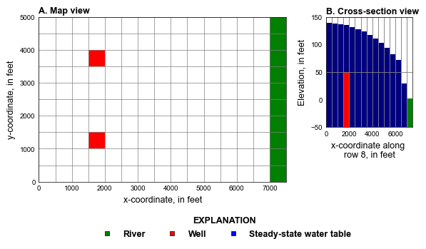
# plot grid
fig = plt.figure(figsize=(6.8, 3.5), constrained_layout=True)
gs = mpl.gridspec.GridSpec(nrows=8, ncols=10, figure=fig, hspace=40, wspace=10)
plt.axis("off")
ax = fig.add_subplot(gs[:7, 0:7])
ax.set_aspect("equal")
mm = flopy.plot.PlotMapView(model=gwf, ax=ax)
mm.plot_bc(ftype="WEL", kper=1, plotAll=True)
mm.plot_bc(ftype="RIV", color="green", plotAll=True)
mm.plot_grid(lw=0.5, color="0.5")
ax.set_ylabel("y-coordinate, in feet")
ax.set_xlabel("x-coordinate, in feet")
styles.heading(ax, letter="A", heading="Map view")
styles.remove_edge_ticks(ax)
ax = fig.add_subplot(gs[:5, 7:])
mm = flopy.plot.PlotCrossSection(model=gwf, ax=ax, line={"row": 7})
mm.plot_array(np.ones((nlay, nrow, ncol)), head=head, cmap="jet")
mm.plot_bc(ftype="WEL", kper=1)
mm.plot_bc(ftype="RIV", color="green", head=head)
mm.plot_grid(lw=0.5, color="0.5")
ax.set_ylabel("Elevation, in feet")
ax.set_xlabel("x-coordinate along \nrow 8, in feet")
styles.heading(ax, letter="B", heading="Cross-section view")
styles.remove_edge_ticks(ax)
# items for legend
ax = fig.add_subplot(gs[7, :])
ax.set_xlim(0, 1)
ax.set_ylim(0, 1)
ax.set_xticks([])
ax.set_yticks([])
ax.spines["top"].set_color("none")
ax.spines["bottom"].set_color("none")
ax.spines["left"].set_color("none")
ax.spines["right"].set_color("none")
ax.patch.set_alpha(0.0)
ax.plot(
-1100, -1100, "s", ms=5, color="green", mec="black", mew=0.5, label="River"
)
ax.plot(
-1100, -1100, "s", ms=5, color="red", mec="black", mew=0.5, label="Well"
)
ax.plot(
-1100,
-1100,
"s",
ms=5,
color="blue",
mec="black",
mew=0.5,
label="Steady-state water table",
)
styles.graph_legend(ax, ncol=3, frameon=False, loc="upper center")
if plot_show:
plt.show()
if plot_save:
fpth = figs_path / f"{sim_name}-grid.png"
fig.savefig(fpth)
# figure with wetdry array
fig = plt.figure(figsize=(4.76, 3), constrained_layout=True)
ax = fig.add_subplot(1, 1, 1)
ax.set_aspect("equal")
mm = flopy.plot.PlotMapView(model=gwf, ax=ax)
wd = mm.plot_array(wetdry_layer0)
mm.plot_grid(lw=0.5, color="0.5")
cbar = plt.colorbar(wd, shrink=0.5)
cbar.ax.set_ylabel("WETDRY parameter")
ax.set_ylabel("y-coordinate, in feet")
ax.set_xlabel("x-coordinate, in feet")
styles.remove_edge_ticks(ax)
if plot_show:
plt.show()
if plot_save:
fig.savefig(figs_path / f"{sim_name}-01.png")
# plot simulated rewetting results
plot_simulated_results(2, gwf, hobj, cobj)
# plot simulated newton results
name = list(parameters.keys())[1]
sim_ws = workspace / name
sim = flopy.mf6.MFSimulation.load(
sim_name=sim_name, sim_ws=sim_ws, verbosity_level=verbosity_level
)
gwf = sim.get_model(sim_name)
# create MODFLOW 6 head object
hobj = gwf.output.head()
# create MODFLOW 6 cell-by-cell budget object
cobj = gwf.output.budget()
# plot the newton results
plot_simulated_results(3, gwf, hobj, cobj)
Running the example
Define a function to run the example scenarios.
[5]:
def scenario(idx, silent=True):
    key = list(parameters.keys())[idx]
    params = parameters[key].copy()
    sim = build_models(key, **params)
    if write:
        write_models(sim, silent=silent)
    if run:
        run_models(sim, silent=silent)
Solve the model by the default means.
[6]:
scenario(0)
<flopy.mf6.data.mfstructure.MFDataItemStructure object at 0x7f863cefdbd0>
run_models took 17.76 ms
Solve the model with the Newton-Raphson formulation.
[7]:
scenario(1)
<flopy.mf6.data.mfstructure.MFDataItemStructure object at 0x7f863cefdbd0>
run_models took 15.95 ms
Plot results.
[8]:
if plot:
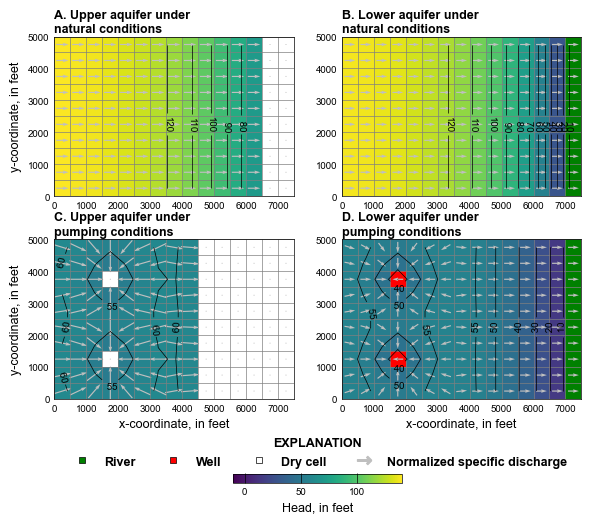
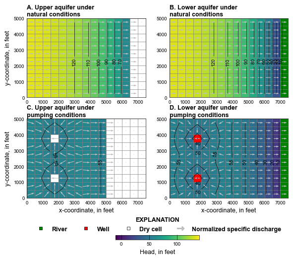
# Simulated water levels and normalized specific discharge vectors in the
# upper and lower aquifers under natural and pumping conditions using (1) the
# rewetting option in the Node Property Flow (NPF) Package with the
# Standard Conductance Formulation and (2) the Newton-Raphson formulation.
# A. Upper aquifer results under natural conditions. B. Lower aquifer results
# under natural conditions C. Upper aquifer results under pumping conditions.
# D. Lower aquifer results under pumping conditions
plot_results()
/home/runner/work/modflow6-examples/modflow6-examples/modflow6-examples/.pixi/envs/default/lib/python3.13/site-packages/IPython/core/pylabtools.py:170: UserWarning: constrained_layout not applied because axes sizes collapsed to zero.  Try making figure larger or Axes decorations smaller.
  fig.canvas.print_figure(bytes_io, **kw)
/tmp/ipykernel_9193/3514210323.py:210: UserWarning: constrained_layout not applied because axes sizes collapsed to zero.  Try making figure larger or Axes decorations smaller.
  fig.savefig(fpth)