This page was generated from
ex-gwt-keating.py.
It's also available as a notebook.
Keating Problem
This problem uses a two-dimensional cross-section model to simulate a perched aquifer overlying a water table aquifer. The presence of a discontinuous low permeability lens causes the perched aquifer to form in response to recharge. The problem also represents solute transport through the system.
Initial setup
Import dependencies, define the example name and workspace, and read settings from environment variables.
[1]:
from pathlib import Path

import flopy
import git
import matplotlib.patches
import matplotlib.pyplot as plt
import numpy as np
import pandas as pd
import pooch
from flopy.plot.styles import styles
from modflow_devtools.misc import get_env, timed

# Example name and workspace paths. If this example is running
# in the git repository, use the folder structure described in
# the README. Otherwise just use the current working directory.
sim_name = "ex-gwt-keating"
try:
    root = Path(git.Repo(".", search_parent_directories=True).working_dir)
except:
    root = None
workspace = root / "examples" if root else Path.cwd()
figs_path = root / "figures" if root else Path.cwd()
data_path = root / "data" / sim_name if root else Path.cwd()

# Settings from environment variables
write = get_env("WRITE", True)
run = get_env("RUN", True)
plot = get_env("PLOT", True)
plot_show = get_env("PLOT_SHOW", True)
plot_save = get_env("PLOT_SAVE", True)
gif_save = get_env("GIF", True)
Define parameters
Define model units, parameters and other settings.
[2]:
# Model units
length_units = "meters"
time_units = "days"

# Model parameters
nlay = 80  # Number of layers
nrow = 1  # Number of rows
ncol = 400  # Number of columns
delr = 25.0  # Column width ($m$)
delc = 1.0  # Row width ($m$)
delz = 25.0  # Layer thickness ($m$)
top = 2000.0  # Top of model domain ($m$)
bottom = 0.0  # Bottom of model domain ($m$)
hka = 1.0e-12  # Permeability of aquifer ($m^2$)
hkc = 1.0e-18  # Permeability of aquitard ($m^2$)
h1 = 800.0  # Head on left side ($m$)
h2 = 100.0  # Head on right side ($m$)
recharge = 0.5  # Recharge ($kg/s$)
recharge_conc = 1.0  # Normalized recharge concentration (unitless)
alpha_l = 1.0  # Longitudinal dispersivity ($m$)
alpha_th = 1.0  # Transverse horizontal dispersivity ($m$)
alpha_tv = 1.0  # Transverse vertical dispersivity ($m$)
period1 = 730  # Length of first simulation period ($d$)
period2 = 29270.0  # Length of second simulation period ($d$)
porosity = 0.1  # Porosity of mobile domain (unitless)
obs1 = (49, 1, 119)  # Layer, row, and column for observation 1
obs2 = (77, 1, 359)  # Layer, row, and column for observation 2

obs1 = tuple(i - 1 for i in obs1)
obs2 = tuple(i - 1 for i in obs2)
seconds_to_days = 24.0 * 60.0 * 60.0
permeability_to_conductivity = 1000.0 * 9.81 / 1.0e-3 * seconds_to_days
hka = hka * permeability_to_conductivity
hkc = hkc * permeability_to_conductivity
botm = [top - (k + 1) * delz for k in range(nlay)]
x = np.arange(0, 10000.0, delr) + delr / 2.0
plotaspect = 1.0

# Fill hydraulic conductivity array
hydraulic_conductivity = np.ones((nlay, nrow, ncol), dtype=float) * hka
for k in range(nlay):
    if 1000.0 <= botm[k] < 1100.0:
        for j in range(ncol):
            if 3000.0 <= x[j] <= 6000.0:
                hydraulic_conductivity[k, 0, j] = hkc

# Calculate recharge by converting from kg/s to m/d
rcol = []
for jcol in range(ncol):
    if 4200.0 <= x[jcol] <= 4800.0:
        rcol.append(jcol)
number_recharge_cells = len(rcol)
rrate = recharge * seconds_to_days / 1000.0
cell_area = delr * delc
rrate = rrate / (float(number_recharge_cells) * cell_area)
rchspd = {}
rchspd[0] = [[(0, 0, j), rrate, recharge_conc] for j in rcol]
rchspd[1] = [[(0, 0, j), rrate, 0.0] for j in rcol]
Model setup
Define functions to build models, write input files, and run the simulation.
[3]:
def build_mf6gwf():
    print(f"Building mf6gwf model...{sim_name}")
    name = "flow"
    sim_ws = workspace / sim_name / "mf6gwf"
    sim = flopy.mf6.MFSimulation(sim_name=name, sim_ws=sim_ws, exe_name="mf6")
    tdis_ds = ((period1, 1, 1.0), (period2, 1, 1.0))
    flopy.mf6.ModflowTdis(
        sim, nper=len(tdis_ds), perioddata=tdis_ds, time_units=time_units
    )
    flopy.mf6.ModflowIms(
        sim,
        print_option="summary",
        complexity="complex",
        no_ptcrecord="all",
        outer_dvclose=1.0e-4,
        outer_maximum=2000,
        under_relaxation="dbd",
        linear_acceleration="BICGSTAB",
        under_relaxation_theta=0.7,
        under_relaxation_kappa=0.08,
        under_relaxation_gamma=0.05,
        under_relaxation_momentum=0.0,
        backtracking_number=20,
        backtracking_tolerance=2.0,
        backtracking_reduction_factor=0.2,
        backtracking_residual_limit=5.0e-4,
        inner_dvclose=1.0e-5,
        rcloserecord="0.0001 relative_rclose",
        inner_maximum=100,
        relaxation_factor=0.0,
        number_orthogonalizations=2,
        preconditioner_levels=8,
        preconditioner_drop_tolerance=0.001,
    )
    gwf = flopy.mf6.ModflowGwf(
        sim, modelname=name, save_flows=True, newtonoptions=["newton"]
    )
    flopy.mf6.ModflowGwfdis(
        gwf,
        length_units=length_units,
        nlay=nlay,
        nrow=nrow,
        ncol=ncol,
        delr=delr,
        delc=delc,
        top=top,
        botm=botm,
    )
    flopy.mf6.ModflowGwfnpf(
        gwf,
        save_specific_discharge=True,
        save_saturation=True,
        save_flows=True,
        icelltype=1,
        k=hydraulic_conductivity,
    )
    flopy.mf6.ModflowGwfic(gwf, strt=600.0)
    chdspd = [[(k, 0, 0), h1] for k in range(nlay) if botm[k] < h1]
    chdspd += [[(k, 0, ncol - 1), h2] for k in range(nlay) if botm[k] < h2]
    flopy.mf6.ModflowGwfchd(
        gwf,
        stress_period_data=chdspd,
        print_input=True,
        print_flows=True,
        save_flows=False,
        pname="CHD-1",
    )
    flopy.mf6.ModflowGwfrch(
        gwf,
        stress_period_data=rchspd,
        auxiliary=["concentration"],
        pname="RCH-1",
    )

    head_filerecord = f"{name}.hds"
    budget_filerecord = f"{name}.bud"
    flopy.mf6.ModflowGwfoc(
        gwf,
        head_filerecord=head_filerecord,
        budget_filerecord=budget_filerecord,
        saverecord=[
            ("HEAD", "ALL"),
            ("BUDGET", "ALL"),
        ],
    )
    return sim


def build_mf6gwt():
    print(f"Building mf6gwt model...{sim_name}")
    name = "trans"
    sim_ws = workspace / sim_name / "mf6gwt"
    sim = flopy.mf6.MFSimulation(
        sim_name=name,
        sim_ws=sim_ws,
        exe_name="mf6",
        continue_=True,
    )
    tdis_ds = ((period1, 73, 1.0), (period2, 2927, 1.0))
    flopy.mf6.ModflowTdis(
        sim, nper=len(tdis_ds), perioddata=tdis_ds, time_units=time_units
    )
    flopy.mf6.ModflowIms(
        sim,
        print_option="summary",
        outer_dvclose=1.0e-4,
        outer_maximum=100,
        under_relaxation="none",
        linear_acceleration="BICGSTAB",
        rcloserecord="1000.0 strict",
        inner_maximum=20,
        inner_dvclose=1.0e-4,
        relaxation_factor=0.0,
        number_orthogonalizations=2,
        preconditioner_levels=8,
        preconditioner_drop_tolerance=0.001,
    )
    gwt = flopy.mf6.ModflowGwt(sim, modelname=name, save_flows=True)
    flopy.mf6.ModflowGwtdis(
        gwt,
        length_units=length_units,
        nlay=nlay,
        nrow=nrow,
        ncol=ncol,
        delr=delr,
        delc=delc,
        top=top,
        botm=botm,
    )
    flopy.mf6.ModflowGwtic(gwt, strt=0)
    flopy.mf6.ModflowGwtmst(gwt, porosity=porosity)
    flopy.mf6.ModflowGwtadv(gwt, scheme="upstream")
    flopy.mf6.ModflowGwtdsp(
        gwt, xt3d_off=True, alh=alpha_l, ath1=alpha_th, atv=alpha_tv
    )
    pd = [
        ("GWFHEAD", "../mf6gwf/flow.hds", None),
        ("GWFBUDGET", "../mf6gwf/flow.bud", None),
    ]
    flopy.mf6.ModflowGwtfmi(gwt, flow_imbalance_correction=True, packagedata=pd)
    sourcerecarray = [
        ("RCH-1", "AUX", "CONCENTRATION"),
    ]
    flopy.mf6.ModflowGwtssm(gwt, sources=sourcerecarray)
    saverecord = {
        0: [
            ("CONCENTRATION", "STEPS", 10),
            ("CONCENTRATION", "LAST"),
            ("CONCENTRATION", "FREQUENCY", 10),
        ],
        1: [
            ("CONCENTRATION", "STEPS", 27, 227),
            ("CONCENTRATION", "LAST"),
            ("CONCENTRATION", "FREQUENCY", 10),
        ],
    }
    flopy.mf6.ModflowGwtoc(
        gwt,
        budget_filerecord=f"{name}.cbc",
        concentration_filerecord=f"{name}.ucn",
        concentrationprintrecord=[
            ("COLUMNS", ncol, "WIDTH", 15, "DIGITS", 6, "GENERAL")
        ],
        saverecord=saverecord,
        printrecord=[
            ("CONCENTRATION", "LAST"),
            ("BUDGET", "ALL"),
        ],
    )
    obs_data = {
        f"{name}.obs.csv": [
            ("obs1", "CONCENTRATION", obs1),
            ("obs2", "CONCENTRATION", obs2),
        ],
    }
    flopy.mf6.ModflowUtlobs(gwt, digits=10, print_input=True, continuous=obs_data)
    return sim


def build_mf6prt():
    print(f"Building mf6prt model...{sim_name}")
    name = "track"
    sim_ws = workspace / sim_name / "mf6prt"
    gwf_ws = workspace / sim_name / "mf6gwf"
    sim = flopy.mf6.MFSimulation(
        sim_name=name,
        sim_ws=sim_ws,
        exe_name="mf6",
        continue_=True,
    )
    tdis_ds = ((period1, 1, 1.0), (period2, 1, 1.0))
    flopy.mf6.ModflowTdis(
        sim, nper=len(tdis_ds), perioddata=tdis_ds, time_units=time_units
    )
    prt = flopy.mf6.ModflowPrt(sim, modelname=name)
    dis = flopy.mf6.ModflowGwtdis(
        prt,
        length_units=length_units,
        nlay=nlay,
        nrow=nrow,
        ncol=ncol,
        delr=delr,
        delc=delc,
        top=top,
        botm=botm,
    )
    mip = flopy.mf6.ModflowPrtmip(prt, pname="mip", porosity=porosity)
    nns = range(prt.modelgrid.ncpl)
    ids = prt.modelgrid.get_lrc(nns)
    ccs = list(
        zip(prt.modelgrid.xcellcenters.ravel(), prt.modelgrid.ycellcenters.ravel())
    )
    prpdata = [
        (nn, *ids[nn], *ccs[nn], 0.5)
        for nn in nns
        if ccs[nn][0] > 4200.0 and ccs[nn][0] < 4800.0
    ]
    prpdata = [(i, *row[1:]) for i, row in enumerate(prpdata)]
    prp = flopy.mf6.ModflowPrtprp(
        prt,
        pname="prp1a",
        filename=f"{name}_1a.prp",
        nreleasepts=len(prpdata),
        packagedata=prpdata,
        releasetimes=[(0,)],
        nreleasetimes=1,
        exit_solve_tolerance=1e-5,
        extend_tracking=False,
        local_z=True,
    )
    budget_record = [f"{name}.cbc"]
    track_record = [f"{name}.trk"]
    trackcsv_record = [f"{name}.trk.csv"]
    flopy.mf6.ModflowPrtoc(
        prt,
        pname="oc",
        budget_filerecord=budget_record,
        track_filerecord=track_record,
        trackcsv_filerecord=trackcsv_record,
        saverecord=[("BUDGET", "ALL")],
    )
    pd = [
        ("GWFGRID", Path(f"../{gwf_ws.name}/flow.dis.grb")),
        ("GWFHEAD", Path(f"../{gwf_ws.name}/flow.hds")),
        ("GWFBUDGET", Path(f"../{gwf_ws.name}/flow.bud")),
    ]
    fmi = flopy.mf6.ModflowPrtfmi(prt, packagedata=pd)
    ems = flopy.mf6.ModflowEms(
        sim,
        pname="ems",
        filename=f"{name}.ems",
    )
    sim.register_solution_package(ems, [prt.name])
    return sim


def build_models():
    sim_mf6gwf = build_mf6gwf()
    sim_mf6gwt = build_mf6gwt()
    sim_mf6prt = build_mf6prt()
    sim_mf2005 = None  # build_mf2005()
    sim_mt3dms = None  # build_mt3dms(sim_mf2005)
    return sim_mf6gwf, sim_mf6gwt, sim_mf6prt, sim_mf2005, sim_mt3dms


def write_models(sims, silent=True):
    sim_mf6gwf, sim_mf6gwt, sim_mf6prt, sim_mf2005, sim_mt3dms = sims
    sim_mf6gwf.write_simulation(silent=silent)
    sim_mf6gwt.write_simulation(silent=silent)
    sim_mf6prt.write_simulation(silent=silent)


@timed
def run_models(sims, silent=True):
    sim_mf6gwf, sim_mf6gwt, sim_mf6prt, sim_mf2005, sim_mt3dms = sims
    success, buff = sim_mf6gwf.run_simulation(silent=silent)
    assert success, buff
    success, buff = sim_mf6gwt.run_simulation(silent=silent)
    assert success, buff
    success, buff = sim_mf6prt.run_simulation(silent=silent)
    assert success, buff
Plotting results
Define functions to plot model results.
[4]:
# Figure properties
figure_size = (7.5, 3)
def plot_results(sims):
print("Plotting model results...")
plot_head_results(sims)
plot_conc_results(sims)
plot_track_results(sims)
plot_cvt_results(sims)
if plot_save and gif_save:
make_animated_gif(sims)
def plot_head_results(sims):
print("Plotting heads...")
sim_mf6gwf, _, _, _, _ = sims
gwf = sim_mf6gwf.flow
botm = gwf.dis.botm.array
with styles.USGSMap():
head = gwf.output.head().get_data()
head = np.where(head > botm, head, np.nan)
fig, ax = plt.subplots(1, 1, figsize=figure_size, dpi=300, tight_layout=True)
pxs = flopy.plot.PlotCrossSection(model=gwf, ax=ax, line={"row": 0})
pa = pxs.plot_array(head, head=head, cmap="jet")
pxs.plot_ibound()
pxs.plot_bc(ftype="RCH", color="red")
pxs.plot_bc(ftype="CHD")
plt.colorbar(pa, shrink=0.5)
confining_rect = matplotlib.patches.Rectangle(
(3000, 1000), 3000, 100, color="gray", alpha=0.5
)
ax.add_patch(confining_rect)
ax.set_xlabel("x position (m)")
ax.set_ylabel("elevation (m)")
ax.set_aspect(plotaspect)
if plot_show:
plt.show()
if plot_save:
sim_folder = sim_mf6gwf.sim_path.parent.name
fname = f"{sim_folder}-head.png"
fpth = figs_path / fname
fig.savefig(fpth)
def plot_track_results(sims):
print("Plotting particle tracks...")
sim_mf6gwf, _, sim_mf6prt, _, _ = sims
gwf = sim_mf6gwf.flow
botm = gwf.dis.botm.array
with styles.USGSMap():
head = gwf.output.head().get_data()
head = np.where(head > botm, head, np.nan)
fig, ax = plt.subplots(1, 1, figsize=figure_size, dpi=300, tight_layout=True)
pxs = flopy.plot.PlotCrossSection(model=gwf, ax=ax, line={"row": 0})
pa = pxs.plot_array(head, head=head, cmap="jet", alpha=0.5)
pxs.plot_ibound()
pxs.plot_bc(ftype="RCH", color="red")
pxs.plot_bc(ftype="CHD")
plt.colorbar(pa, shrink=0.5)
confining_rect = matplotlib.patches.Rectangle(
(3000, 1000), 3000, 100, color="gray", alpha=0.5
)
ax.add_patch(confining_rect)
ax.set_xlabel("x position (m)")
ax.set_ylabel("elevation (m)")
ax.set_aspect(plotaspect)
pathlines = pd.read_csv(sim_mf6prt.sim_path / "track.trk.csv")
for _, pl in pathlines.groupby("irpt"):
pl.plot("x", "z", lw=0.2, ax=ax, alpha=0.4, legend=False)
if plot_show:
plt.show()
if plot_save:
sim_folder = sim_mf6prt.sim_path.parent.name
fname = f"{sim_folder}-tracks.png"
fpth = figs_path / fname
fig.savefig(fpth)
def plot_conc_results(sims):
print("Plotting concentrations...")
sim_mf6gwf, sim_mf6gwt, _, _, _ = sims
gwf = sim_mf6gwf.flow
gwt = sim_mf6gwt.trans
botm = gwf.dis.botm.array
with styles.USGSMap():
head = gwf.output.head().get_data()
head = np.where(head > botm, head, np.nan)
sim_ws = Path(sim_mf6gwt.simulation_data.mfpath.get_sim_path())
cobj = gwt.output.concentration()
conc_times = cobj.get_times()
conc_times = np.array(conc_times)
fig, axes = plt.subplots(3, 1, figsize=(7.5, 4.5), dpi=300, tight_layout=True)
xgrid, _, zgrid = gwt.modelgrid.xyzcellcenters
# Desired plot times
plot_times = [100.0, 1000.0, 3000.0]
nplots = len(plot_times)
for iplot in range(nplots):
print(f" Plotting conc {iplot + 1}")
time_in_pub = plot_times[iplot]
idx_conc = (np.abs(conc_times - time_in_pub)).argmin()
totim = conc_times[idx_conc]
ax = axes[iplot]
pxs = flopy.plot.PlotCrossSection(model=gwf, ax=ax, line={"row": 0})
conc = cobj.get_data(totim=totim)
conc = np.where(head > botm, conc, np.nan)
pa = pxs.plot_array(conc, head=head, cmap="jet", vmin=0, vmax=1.0)
pxs.plot_bc(ftype="RCH", color="red")
pxs.plot_bc(ftype="CHD")
confining_rect = matplotlib.patches.Rectangle(
(3000, 1000), 3000, 100, color="gray", alpha=0.5
)
ax.add_patch(confining_rect)
if iplot == 2:
ax.set_xlabel("x position (m)")
ax.set_ylabel("elevation (m)")
title = f"Time = {totim}"
letter = chr(ord("@") + iplot + 1)
styles.heading(letter=letter, heading=title, ax=ax)
ax.set_aspect(plotaspect)
for k, i, j in [obs1, obs2]:
x = xgrid[i, j]
z = zgrid[k, i, j]
ax.plot(
x,
z,
markerfacecolor="yellow",
markeredgecolor="black",
marker="o",
markersize="4",
)
if plot_show:
plt.show()
if plot_save:
sim_folder = sim_ws.parent.name
fname = f"{sim_folder}-conc.png"
fpth = figs_path / fname
fig.savefig(fpth)
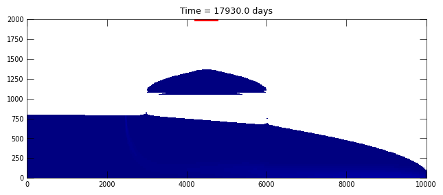
def make_animated_gif(sims):
import copy
import matplotlib as mpl
from matplotlib.animation import FuncAnimation, PillowWriter
print("Animating concentrations...")
sim_mf6gwf, sim_mf6gwt, _, _, _ = sims
gwf = sim_mf6gwf.flow
gwt = sim_mf6gwt.trans
botm = gwf.dis.botm.array
# load head
with styles.USGSMap() as fs:
head = gwf.output.head().get_data()
head = np.where(head > botm, head, np.nan)
# load concentration
cobj = gwt.output.concentration()
conc_times = cobj.get_times()
conc_times = np.array(conc_times)
conc = cobj.get_alldata()
# set up the figure
fig = plt.figure(figsize=(7.5, 3))
ax = fig.add_subplot(1, 1, 1)
pxs = flopy.plot.PlotCrossSection(
model=gwf,
ax=ax,
line={"row": 0},
extent=(0, 10000, 0, 2000),
)
cmap = copy.copy(mpl.colormaps["jet"])
cmap.set_bad("white")
nodata = -999.0
a = np.where(head > botm, conc[0], nodata)
a = np.ma.masked_where(a < 0, a)
pc = pxs.plot_array(a, head=head, cmap=cmap, vmin=0, vmax=1)
pxs.plot_bc(ftype="RCH", color="red")
pxs.plot_bc(ftype="CHD")
def init():
ax.set_title(f"Time = {conc_times[0]} days")
def update(i):
a = np.where(head > botm, conc[i], nodata)
a = np.ma.masked_where(a < 0, a)
a = a[~a.mask]
pc.set_array(a.flatten())
ax.set_title(f"Time = {conc_times[i]} days")
# Stop the animation at 18,000 days
idx_end = (np.abs(conc_times - 18000.0)).argmin()
ani = FuncAnimation(fig, update, range(1, idx_end), init_func=init)
writer = PillowWriter(fps=25)
fpth = figs_path / f"{sim_name}.gif"
ani.save(fpth, writer=writer)
def plot_cvt_results(sims):
print("Plotting cvt model results...")
_, sim_mf6gwt, _, _, _ = sims
gwt = sim_mf6gwt.trans
with styles.USGSMap():
sim_ws = Path(sim_mf6gwt.simulation_data.mfpath.get_sim_path())
mf6gwt_ra = gwt.obs.output.obs().data
dt = [("totim", "f8"), ("obs", "f8")]
fname = "keating_obs1.csv"
fpath = pooch.retrieve(
url=f"https://github.com/MODFLOW-ORG/modflow6-examples/raw/master/data/{sim_name}/{fname}",
fname=fname,
path=data_path,
known_hash="md5:174c5548c3bbb9ea4ebc8b5a33ea2851",
)
obs1ra = np.genfromtxt(fpath, delimiter=",", deletechars="", dtype=dt)
fname = "keating_obs2.csv"
fpath = pooch.retrieve(
url=f"https://github.com/MODFLOW-ORG/modflow6-examples/raw/master/data/{sim_name}/{fname}",
fname=fname,
path=data_path,
known_hash="md5:8de2ef529a2537ecd6c62bc207b67fb5",
)
obs2ra = np.genfromtxt(fpath, delimiter=",", deletechars="", dtype=dt)
fig, axes = plt.subplots(2, 1, figsize=(6, 4), dpi=300, tight_layout=True)
ax = axes[0]
ax.plot(
mf6gwt_ra["totim"], mf6gwt_ra["OBS1"], "b-", alpha=1.0, label="MODFLOW 6"
)
ax.plot(
obs1ra["totim"],
obs1ra["obs"],
markerfacecolor="None",
markeredgecolor="k",
marker="o",
markersize="4",
linestyle="None",
label="Keating and Zyvolosky (2009)",
)
ax.set_xlim(0, 8000)
ax.set_ylim(0, 0.80)
ax.set_xlabel("time, in days")
ax.set_ylabel("normalized concentration, unitless")
styles.graph_legend(ax)
ax = axes[1]
ax.plot(
mf6gwt_ra["totim"], mf6gwt_ra["OBS2"], "b-", alpha=1.0, label="MODFLOW 6"
)
ax.plot(
obs2ra["totim"],
obs2ra["obs"],
markerfacecolor="None",
markeredgecolor="k",
marker="o",
markersize="4",
linestyle="None",
label="Keating and Zyvolosky (2009)",
)
ax.set_xlim(0, 30000)
ax.set_ylim(0, 0.20)
ax.set_xlabel("time, in days")
ax.set_ylabel("normalized concentration, unitless")
styles.graph_legend(ax)
if plot_show:
plt.show()
if plot_save:
sim_folder = sim_ws.parent.name
fname = f"{sim_folder}-cvt.png"
fpth = figs_path / fname
fig.savefig(fpth)
Running the example
Define and invoke a function to run the example scenario, then plot results.
[5]:
def scenario(silent=True):
    sim = build_models()
    if write:
        write_models(sim, silent=silent)
    if run:
        run_models(sim, silent=silent)
    if plot:
        plot_results(sim)


scenario(silent=False)
Building mf6gwf model...ex-gwt-keating
<flopy.mf6.data.mfstructure.MFDataItemStructure object at 0x7f22b30f4f50>
Building mf6gwt model...ex-gwt-keating
<flopy.mf6.data.mfstructure.MFDataItemStructure object at 0x7f22b30f4f50>
Building mf6prt model...ex-gwt-keating
writing simulation...
  writing simulation name file...
  writing simulation tdis package...
  writing solution package ims_-1...
  writing model flow...
    writing model name file...
    writing package dis...
    writing package npf...
    writing package ic...
    writing package chd-1...
INFORMATION: maxbound in ('', 'chd', 'dimensions') changed to 36 based on size of stress_period_data
    writing package rch-1...
INFORMATION: maxbound in ('', 'rch', 'dimensions') changed to 24 based on size of stress_period_data
    writing package oc...
writing simulation...
  writing simulation name file...
  writing simulation tdis package...
  writing solution package ims_-1...
  writing model trans...
    writing model name file...
    writing package dis...
    writing package ic...
    writing package mst...
    writing package adv...
    writing package dsp...
    writing package fmi...
    writing package ssm...
    writing package oc...
    writing package obs_0...
writing simulation...
  writing simulation name file...
  writing simulation tdis package...
  writing solution package ems...
  writing model track...
    writing model name file...
    writing package dis...
    writing package mip...
    writing package prp1a...
    writing package oc...
    writing package fmi...
FloPy is using the following executable to run the model: ../../../../../../../.local/bin/modflow/mf6
                                   MODFLOW 6
                U.S. GEOLOGICAL SURVEY MODULAR HYDROLOGIC MODEL
                  VERSION 6.8.0.dev0 (preliminary) 02/06/2026
                               ***DEVELOP MODE***

        MODFLOW 6 compiled Feb 15 2026 14:55:26 with GCC version 13.3.0

This software is preliminary or provisional and is subject to
revision. It is being provided to meet the need for timely best
science. The software has not received final approval by the U.S.
Geological Survey (USGS). No warranty, expressed or implied, is made
by the USGS or the U.S. Government as to the functionality of the
software and related material nor shall the fact of release
constitute any such warranty. The software is provided on the
condition that neither the USGS nor the U.S. Government shall be held
liable for any damages resulting from the authorized or unauthorized
use of the software.


 MODFLOW runs in SEQUENTIAL mode

 Run start date and time (yyyy/mm/dd hh:mm:ss): 2026/02/15 15:04:39

 Writing simulation list file: mfsim.lst
 Using Simulation name file: mfsim.nam

    Solving:  Stress period:     1    Time step:     1
    Solving:  Stress period:     2    Time step:     1

 Run end date and time (yyyy/mm/dd hh:mm:ss): 2026/02/15 15:04:45
 Elapsed run time:  5.366 Seconds

 Normal termination of simulation.
FloPy is using the following executable to run the model: ../../../../../../../.local/bin/modflow/mf6
                                   MODFLOW 6
                U.S. GEOLOGICAL SURVEY MODULAR HYDROLOGIC MODEL
                  VERSION 6.8.0.dev0 (preliminary) 02/06/2026
                               ***DEVELOP MODE***

        MODFLOW 6 compiled Feb 15 2026 14:55:26 with GCC version 13.3.0

This software is preliminary or provisional and is subject to
revision. It is being provided to meet the need for timely best
science. The software has not received final approval by the U.S.
Geological Survey (USGS). No warranty, expressed or implied, is made
by the USGS or the U.S. Government as to the functionality of the
software and related material nor shall the fact of release
constitute any such warranty. The software is provided on the
condition that neither the USGS nor the U.S. Government shall be held
liable for any damages resulting from the authorized or unauthorized
use of the software.


 MODFLOW runs in SEQUENTIAL mode

 Run start date and time (yyyy/mm/dd hh:mm:ss): 2026/02/15 15:04:45

 Writing simulation list file: mfsim.lst
 Using Simulation name file: mfsim.nam

    Solving:  Stress period:     1    Time step:     1
    Solving:  Stress period:     1    Time step:     2
    Solving:  Stress period:     1    Time step:     3
    Solving:  Stress period:     1    Time step:     4
    Solving:  Stress period:     1    Time step:     5
    Solving:  Stress period:     1    Time step:     6
    Solving:  Stress period:     1    Time step:     7
    Solving:  Stress period:     1    Time step:     8
    Solving:  Stress period:     1    Time step:     9
    Solving:  Stress period:     1    Time step:    10
    Solving:  Stress period:     1    Time step:    11
    Solving:  Stress period:     1    Time step:    12
    Solving:  Stress period:     1    Time step:    13
    Solving:  Stress period:     1    Time step:    14
    Solving:  Stress period:     1    Time step:    15
    Solving:  Stress period:     1    Time step:    16
    Solving:  Stress period:     1    Time step:    17
    Solving:  Stress period:     1    Time step:    18
    Solving:  Stress period:     1    Time step:    19
    Solving:  Stress period:     1    Time step:    20
    Solving:  Stress period:     1    Time step:    21
    Solving:  Stress period:     1    Time step:    22
    Solving:  Stress period:     1    Time step:    23
    Solving:  Stress period:     1    Time step:    24
    Solving:  Stress period:     1    Time step:    25
    Solving:  Stress period:     1    Time step:    26
    Solving:  Stress period:     1    Time step:    27
    Solving:  Stress period:     1    Time step:    28
    Solving:  Stress period:     1    Time step:    29
    Solving:  Stress period:     1    Time step:    30
    Solving:  Stress period:     1    Time step:    31
    Solving:  Stress period:     1    Time step:    32
    Solving:  Stress period:     1    Time step:    33
    Solving:  Stress period:     1    Time step:    34
    Solving:  Stress period:     1    Time step:    35
    Solving:  Stress period:     1    Time step:    36
    Solving:  Stress period:     1    Time step:    37
    Solving:  Stress period:     1    Time step:    38
    Solving:  Stress period:     1    Time step:    39
    Solving:  Stress period:     1    Time step:    40
    Solving:  Stress period:     1    Time step:    41
    Solving:  Stress period:     1    Time step:    42
    Solving:  Stress period:     1    Time step:    43
    Solving:  Stress period:     1    Time step:    44
    Solving:  Stress period:     1    Time step:    45
    Solving:  Stress period:     1    Time step:    46
    Solving:  Stress period:     1    Time step:    47
    Solving:  Stress period:     1    Time step:    48
    Solving:  Stress period:     1    Time step:    49
    Solving:  Stress period:     1    Time step:    50
    Solving:  Stress period:     1    Time step:    51
    Solving:  Stress period:     1    Time step:    52
    Solving:  Stress period:     1    Time step:    53
    Solving:  Stress period:     1    Time step:    54
    Solving:  Stress period:     1    Time step:    55
    Solving:  Stress period:     1    Time step:    56
    Solving:  Stress period:     1    Time step:    57
    Solving:  Stress period:     1    Time step:    58
    Solving:  Stress period:     1    Time step:    59
    Solving:  Stress period:     1    Time step:    60
    Solving:  Stress period:     1    Time step:    61
    Solving:  Stress period:     1    Time step:    62
    Solving:  Stress period:     1    Time step:    63
    Solving:  Stress period:     1    Time step:    64
    Solving:  Stress period:     1    Time step:    65
    Solving:  Stress period:     1    Time step:    66
    Solving:  Stress period:     1    Time step:    67
    Solving:  Stress period:     1    Time step:    68
    Solving:  Stress period:     1    Time step:    69
    Solving:  Stress period:     1    Time step:    70
    Solving:  Stress period:     1    Time step:    71
    Solving:  Stress period:     1    Time step:    72
    Solving:  Stress period:     1    Time step:    73
    Solving:  Stress period:     2    Time step:     1
    Solving:  Stress period:     2    Time step:     2
    Solving:  Stress period:     2    Time step:     3
    Solving:  Stress period:     2    Time step:     4
    Solving:  Stress period:     2    Time step:     5
    Solving:  Stress period:     2    Time step:     6
    Solving:  Stress period:     2    Time step:     7
    Solving:  Stress period:     2    Time step:     8
    Solving:  Stress period:     2    Time step:     9
    Solving:  Stress period:     2    Time step:    10
    Solving:  Stress period:     2    Time step:    11
    Solving:  Stress period:     2    Time step:    12
    Solving:  Stress period:     2    Time step:    13
    Solving:  Stress period:     2    Time step:    14
    Solving:  Stress period:     2    Time step:    15
    Solving:  Stress period:     2    Time step:    16
    Solving:  Stress period:     2    Time step:    17
    Solving:  Stress period:     2    Time step:    18
    Solving:  Stress period:     2    Time step:    19
    Solving:  Stress period:     2    Time step:    20
    Solving:  Stress period:     2    Time step:    21
    Solving:  Stress period:     2    Time step:    22
    Solving:  Stress period:     2    Time step:    23
    Solving:  Stress period:     2    Time step:    24
    Solving:  Stress period:     2    Time step:    25
    Solving:  Stress period:     2    Time step:    26
    Solving:  Stress period:     2    Time step:    27
    Solving:  Stress period:     2    Time step:    28
    Solving:  Stress period:     2    Time step:    29
    Solving:  Stress period:     2    Time step:    30
    Solving:  Stress period:     2    Time step:    31
    Solving:  Stress period:     2    Time step:    32
    Solving:  Stress period:     2    Time step:    33
    Solving:  Stress period:     2    Time step:    34
    Solving:  Stress period:     2    Time step:    35
    Solving:  Stress period:     2    Time step:    36
    Solving:  Stress period:     2    Time step:    37
    Solving:  Stress period:     2    Time step:    38
    Solving:  Stress period:     2    Time step:    39
    Solving:  Stress period:     2    Time step:    40
    Solving:  Stress period:     2    Time step:    41
    Solving:  Stress period:     2    Time step:    42
    Solving:  Stress period:     2    Time step:    43
    Solving:  Stress period:     2    Time step:    44
    Solving:  Stress period:     2    Time step:    45
    Solving:  Stress period:     2    Time step:    46
    Solving:  Stress period:     2    Time step:    47
    Solving:  Stress period:     2    Time step:    48
    Solving:  Stress period:     2    Time step:    49
    Solving:  Stress period:     2    Time step:    50
    Solving:  Stress period:     2    Time step:    51
    Solving:  Stress period:     2    Time step:    52
    Solving:  Stress period:     2    Time step:    53
    Solving:  Stress period:     2    Time step:    54
    Solving:  Stress period:     2    Time step:    55
    Solving:  Stress period:     2    Time step:    56
    Solving:  Stress period:     2    Time step:    57
    Solving:  Stress period:     2    Time step:    58
    Solving:  Stress period:     2    Time step:    59
    Solving:  Stress period:     2    Time step:    60
    Solving:  Stress period:     2    Time step:    61
    Solving:  Stress period:     2    Time step:    62
    Solving:  Stress period:     2    Time step:    63
    Solving:  Stress period:     2    Time step:    64
    Solving:  Stress period:     2    Time step:    65
    Solving:  Stress period:     2    Time step:    66
    Solving:  Stress period:     2    Time step:    67
    Solving:  Stress period:     2    Time step:    68
    Solving:  Stress period:     2    Time step:    69
    Solving:  Stress period:     2    Time step:    70
    Solving:  Stress period:     2    Time step:    71
    Solving:  Stress period:     2    Time step:    72
    Solving:  Stress period:     2    Time step:    73
    Solving:  Stress period:     2    Time step:    74
    Solving:  Stress period:     2    Time step:    75
    Solving:  Stress period:     2    Time step:    76
    Solving:  Stress period:     2    Time step:    77
    Solving:  Stress period:     2    Time step:    78
    Solving:  Stress period:     2    Time step:    79
    Solving:  Stress period:     2    Time step:    80
    Solving:  Stress period:     2    Time step:    81
    Solving:  Stress period:     2    Time step:    82
    Solving:  Stress period:     2    Time step:    83
    Solving:  Stress period:     2    Time step:    84
    Solving:  Stress period:     2    Time step:    85
    Solving:  Stress period:     2    Time step:    86
    Solving:  Stress period:     2    Time step:    87
    Solving:  Stress period:     2    Time step:    88
    Solving:  Stress period:     2    Time step:    89
    Solving:  Stress period:     2    Time step:    90
    Solving:  Stress period:     2    Time step:    91
    Solving:  Stress period:     2    Time step:    92
    Solving:  Stress period:     2    Time step:    93
    Solving:  Stress period:     2    Time step:    94
    Solving:  Stress period:     2    Time step:    95
    Solving:  Stress period:     2    Time step:    96
    Solving:  Stress period:     2    Time step:    97
    Solving:  Stress period:     2    Time step:    98
    Solving:  Stress period:     2    Time step:    99
    Solving:  Stress period:     2    Time step:   100
    Solving:  Stress period:     2    Time step:   101
    Solving:  Stress period:     2    Time step:   102
    Solving:  Stress period:     2    Time step:   103
    Solving:  Stress period:     2    Time step:   104
    Solving:  Stress period:     2    Time step:   105
    Solving:  Stress period:     2    Time step:   106
    Solving:  Stress period:     2    Time step:   107
    Solving:  Stress period:     2    Time step:   108
    Solving:  Stress period:     2    Time step:   109
    Solving:  Stress period:     2    Time step:   110
    Solving:  Stress period:     2    Time step:   111
    Solving:  Stress period:     2    Time step:   112
    Solving:  Stress period:     2    Time step:   113
    Solving:  Stress period:     2    Time step:   114
    Solving:  Stress period:     2    Time step:   115
    Solving:  Stress period:     2    Time step:   116
    Solving:  Stress period:     2    Time step:   117
    Solving:  Stress period:     2    Time step:   118
    Solving:  Stress period:     2    Time step:   119
    Solving:  Stress period:     2    Time step:   120
    Solving:  Stress period:     2    Time step:   121
    Solving:  Stress period:     2    Time step:   122
    Solving:  Stress period:     2    Time step:   123
    Solving:  Stress period:     2    Time step:   124
    Solving:  Stress period:     2    Time step:   125
    Solving:  Stress period:     2    Time step:   126
    Solving:  Stress period:     2    Time step:   127
    Solving:  Stress period:     2    Time step:   128
    Solving:  Stress period:     2    Time step:   129
    Solving:  Stress period:     2    Time step:   130
    Solving:  Stress period:     2    Time step:   131
    Solving:  Stress period:     2    Time step:   132
    Solving:  Stress period:     2    Time step:   133
    Solving:  Stress period:     2    Time step:   134
    Solving:  Stress period:     2    Time step:   135
    Solving:  Stress period:     2    Time step:   136
    Solving:  Stress period:     2    Time step:   137
    Solving:  Stress period:     2    Time step:   138
    Solving:  Stress period:     2    Time step:   139
    Solving:  Stress period:     2    Time step:   140
    Solving:  Stress period:     2    Time step:   141
    Solving:  Stress period:     2    Time step:   142
    Solving:  Stress period:     2    Time step:   143
    Solving:  Stress period:     2    Time step:   144
    Solving:  Stress period:     2    Time step:   145
    Solving:  Stress period:     2    Time step:   146
    Solving:  Stress period:     2    Time step:   147
    Solving:  Stress period:     2    Time step:   148
    Solving:  Stress period:     2    Time step:   149
    Solving:  Stress period:     2    Time step:   150
    Solving:  Stress period:     2    Time step:   151
    Solving:  Stress period:     2    Time step:   152
    Solving:  Stress period:     2    Time step:   153
    Solving:  Stress period:     2    Time step:   154
    Solving:  Stress period:     2    Time step:   155
    Solving:  Stress period:     2    Time step:   156
    Solving:  Stress period:     2    Time step:   157
    Solving:  Stress period:     2    Time step:   158
    Solving:  Stress period:     2    Time step:   159
    Solving:  Stress period:     2    Time step:   160
    Solving:  Stress period:     2    Time step:   161
    Solving:  Stress period:     2    Time step:   162
    Solving:  Stress period:     2    Time step:   163
    Solving:  Stress period:     2    Time step:   164
    Solving:  Stress period:     2    Time step:   165
    Solving:  Stress period:     2    Time step:   166
    Solving:  Stress period:     2    Time step:   167
    Solving:  Stress period:     2    Time step:   168
    Solving:  Stress period:     2    Time step:   169
    Solving:  Stress period:     2    Time step:   170
    Solving:  Stress period:     2    Time step:   171
    Solving:  Stress period:     2    Time step:   172
    Solving:  Stress period:     2    Time step:   173
    Solving:  Stress period:     2    Time step:   174
    Solving:  Stress period:     2    Time step:   175
    Solving:  Stress period:     2    Time step:   176
    Solving:  Stress period:     2    Time step:   177
    Solving:  Stress period:     2    Time step:   178
    Solving:  Stress period:     2    Time step:   179
    Solving:  Stress period:     2    Time step:   180
    Solving:  Stress period:     2    Time step:   181
    Solving:  Stress period:     2    Time step:   182
    Solving:  Stress period:     2    Time step:   183
    Solving:  Stress period:     2    Time step:   184
    Solving:  Stress period:     2    Time step:   185
    Solving:  Stress period:     2    Time step:   186
    Solving:  Stress period:     2    Time step:   187
    Solving:  Stress period:     2    Time step:   188
    Solving:  Stress period:     2    Time step:   189
    Solving:  Stress period:     2    Time step:   190
    Solving:  Stress period:     2    Time step:   191
    Solving:  Stress period:     2    Time step:   192
    Solving:  Stress period:     2    Time step:   193
    Solving:  Stress period:     2    Time step:   194
    Solving:  Stress period:     2    Time step:   195
    Solving:  Stress period:     2    Time step:   196
    Solving:  Stress period:     2    Time step:   197
    Solving:  Stress period:     2    Time step:   198
    Solving:  Stress period:     2    Time step:   199
    Solving:  Stress period:     2    Time step:   200
    Solving:  Stress period:     2    Time step:   201
    Solving:  Stress period:     2    Time step:   202
    Solving:  Stress period:     2    Time step:   203
    Solving:  Stress period:     2    Time step:   204
    Solving:  Stress period:     2    Time step:   205
    Solving:  Stress period:     2    Time step:   206
    Solving:  Stress period:     2    Time step:   207
    Solving:  Stress period:     2    Time step:   208
    Solving:  Stress period:     2    Time step:   209
    Solving:  Stress period:     2    Time step:   210
    Solving:  Stress period:     2    Time step:   211
    Solving:  Stress period:     2    Time step:   212
    Solving:  Stress period:     2    Time step:   213
    Solving:  Stress period:     2    Time step:   214
    Solving:  Stress period:     2    Time step:   215
    Solving:  Stress period:     2    Time step:   216
    Solving:  Stress period:     2    Time step:   217
    Solving:  Stress period:     2    Time step:   218
    Solving:  Stress period:     2    Time step:   219
    Solving:  Stress period:     2    Time step:   220
    Solving:  Stress period:     2    Time step:   221
    Solving:  Stress period:     2    Time step:   222
    Solving:  Stress period:     2    Time step:   223
    Solving:  Stress period:     2    Time step:   224
    Solving:  Stress period:     2    Time step:   225
    Solving:  Stress period:     2    Time step:   226
    Solving:  Stress period:     2    Time step:   227
    Solving:  Stress period:     2    Time step:   228
    Solving:  Stress period:     2    Time step:   229
    Solving:  Stress period:     2    Time step:   230
    Solving:  Stress period:     2    Time step:   231
    Solving:  Stress period:     2    Time step:   232
    Solving:  Stress period:     2    Time step:   233
    Solving:  Stress period:     2    Time step:   234
    Solving:  Stress period:     2    Time step:   235
    Solving:  Stress period:     2    Time step:   236
    Solving:  Stress period:     2    Time step:   237
    Solving:  Stress period:     2    Time step:   238
    Solving:  Stress period:     2    Time step:   239
    Solving:  Stress period:     2    Time step:   240
    Solving:  Stress period:     2    Time step:   241
    Solving:  Stress period:     2    Time step:   242
    Solving:  Stress period:     2    Time step:   243
    Solving:  Stress period:     2    Time step:   244
    Solving:  Stress period:     2    Time step:   245
    Solving:  Stress period:     2    Time step:   246
    Solving:  Stress period:     2    Time step:   247
    Solving:  Stress period:     2    Time step:   248
    Solving:  Stress period:     2    Time step:   249
    Solving:  Stress period:     2    Time step:   250
    Solving:  Stress period:     2    Time step:   251
    Solving:  Stress period:     2    Time step:   252
    Solving:  Stress period:     2    Time step:   253
    Solving:  Stress period:     2    Time step:   254
    Solving:  Stress period:     2    Time step:   255
    Solving:  Stress period:     2    Time step:   256
    Solving:  Stress period:     2    Time step:   257
    Solving:  Stress period:     2    Time step:   258
    Solving:  Stress period:     2    Time step:   259
    Solving:  Stress period:     2    Time step:   260
    Solving:  Stress period:     2    Time step:   261
    Solving:  Stress period:     2    Time step:   262
    Solving:  Stress period:     2    Time step:   263
    Solving:  Stress period:     2    Time step:   264
    Solving:  Stress period:     2    Time step:   265
    Solving:  Stress period:     2    Time step:   266
    Solving:  Stress period:     2    Time step:   267
    Solving:  Stress period:     2    Time step:   268
    Solving:  Stress period:     2    Time step:   269
    Solving:  Stress period:     2    Time step:   270
    Solving:  Stress period:     2    Time step:   271
    Solving:  Stress period:     2    Time step:   272
    Solving:  Stress period:     2    Time step:   273
    Solving:  Stress period:     2    Time step:   274
    Solving:  Stress period:     2    Time step:   275
    Solving:  Stress period:     2    Time step:   276
    Solving:  Stress period:     2    Time step:   277
    Solving:  Stress period:     2    Time step:   278
    Solving:  Stress period:     2    Time step:   279
    Solving:  Stress period:     2    Time step:   280
    Solving:  Stress period:     2    Time step:   281
    Solving:  Stress period:     2    Time step:   282
    Solving:  Stress period:     2    Time step:   283
    Solving:  Stress period:     2    Time step:   284
    Solving:  Stress period:     2    Time step:   285
    Solving:  Stress period:     2    Time step:   286
    Solving:  Stress period:     2    Time step:   287
    Solving:  Stress period:     2    Time step:   288
    Solving:  Stress period:     2    Time step:   289
    Solving:  Stress period:     2    Time step:   290
    Solving:  Stress period:     2    Time step:   291
    Solving:  Stress period:     2    Time step:   292
    Solving:  Stress period:     2    Time step:   293
    Solving:  Stress period:     2    Time step:   294
    Solving:  Stress period:     2    Time step:   295
    Solving:  Stress period:     2    Time step:   296
    Solving:  Stress period:     2    Time step:   297
    Solving:  Stress period:     2    Time step:   298
    Solving:  Stress period:     2    Time step:   299
    Solving:  Stress period:     2    Time step:   300
    Solving:  Stress period:     2    Time step:   301
    Solving:  Stress period:     2    Time step:   302
    Solving:  Stress period:     2    Time step:   303
    Solving:  Stress period:     2    Time step:   304
    Solving:  Stress period:     2    Time step:   305
    Solving:  Stress period:     2    Time step:   306
    Solving:  Stress period:     2    Time step:   307
    Solving:  Stress period:     2    Time step:   308
    Solving:  Stress period:     2    Time step:   309
    Solving:  Stress period:     2    Time step:   310
    Solving:  Stress period:     2    Time step:   311
    Solving:  Stress period:     2    Time step:   312
    Solving:  Stress period:     2    Time step:   313
    Solving:  Stress period:     2    Time step:   314
    Solving:  Stress period:     2    Time step:   315
    Solving:  Stress period:     2    Time step:   316
    Solving:  Stress period:     2    Time step:   317
    Solving:  Stress period:     2    Time step:   318
    Solving:  Stress period:     2    Time step:   319
    Solving:  Stress period:     2    Time step:   320
    Solving:  Stress period:     2    Time step:   321
    Solving:  Stress period:     2    Time step:   322
    Solving:  Stress period:     2    Time step:   323
    Solving:  Stress period:     2    Time step:   324
    Solving:  Stress period:     2    Time step:   325
    Solving:  Stress period:     2    Time step:   326
    Solving:  Stress period:     2    Time step:   327
    Solving:  Stress period:     2    Time step:   328
    Solving:  Stress period:     2    Time step:   329
    Solving:  Stress period:     2    Time step:   330
    Solving:  Stress period:     2    Time step:   331
    Solving:  Stress period:     2    Time step:   332
    Solving:  Stress period:     2    Time step:   333
    Solving:  Stress period:     2    Time step:   334
    Solving:  Stress period:     2    Time step:   335
    Solving:  Stress period:     2    Time step:   336
    Solving:  Stress period:     2    Time step:   337
    Solving:  Stress period:     2    Time step:   338
    Solving:  Stress period:     2    Time step:   339
    Solving:  Stress period:     2    Time step:   340
    Solving:  Stress period:     2    Time step:   341
    Solving:  Stress period:     2    Time step:   342
    Solving:  Stress period:     2    Time step:   343
    Solving:  Stress period:     2    Time step:   344
    Solving:  Stress period:     2    Time step:   345
    Solving:  Stress period:     2    Time step:   346
    Solving:  Stress period:     2    Time step:   347
    Solving:  Stress period:     2    Time step:   348
    Solving:  Stress period:     2    Time step:   349
    Solving:  Stress period:     2    Time step:   350
    Solving:  Stress period:     2    Time step:   351
    Solving:  Stress period:     2    Time step:   352
    Solving:  Stress period:     2    Time step:   353
    Solving:  Stress period:     2    Time step:   354
    Solving:  Stress period:     2    Time step:   355
    Solving:  Stress period:     2    Time step:   356
    Solving:  Stress period:     2    Time step:   357
    Solving:  Stress period:     2    Time step:   358
    Solving:  Stress period:     2    Time step:   359
    Solving:  Stress period:     2    Time step:   360
    Solving:  Stress period:     2    Time step:   361
    Solving:  Stress period:     2    Time step:   362
    Solving:  Stress period:     2    Time step:   363
    Solving:  Stress period:     2    Time step:   364
    Solving:  Stress period:     2    Time step:   365
    Solving:  Stress period:     2    Time step:   366
    Solving:  Stress period:     2    Time step:   367
    Solving:  Stress period:     2    Time step:   368
    Solving:  Stress period:     2    Time step:   369
    Solving:  Stress period:     2    Time step:   370
    Solving:  Stress period:     2    Time step:   371
    Solving:  Stress period:     2    Time step:   372
    Solving:  Stress period:     2    Time step:   373
    Solving:  Stress period:     2    Time step:   374
    Solving:  Stress period:     2    Time step:   375
    Solving:  Stress period:     2    Time step:   376
    Solving:  Stress period:     2    Time step:   377
    Solving:  Stress period:     2    Time step:   378
    Solving:  Stress period:     2    Time step:   379
    Solving:  Stress period:     2    Time step:   380
    Solving:  Stress period:     2    Time step:   381
    Solving:  Stress period:     2    Time step:   382
    Solving:  Stress period:     2    Time step:   383
    Solving:  Stress period:     2    Time step:   384
    Solving:  Stress period:     2    Time step:   385
    Solving:  Stress period:     2    Time step:   386
    Solving:  Stress period:     2    Time step:   387
    Solving:  Stress period:     2    Time step:   388
    Solving:  Stress period:     2    Time step:   389
    Solving:  Stress period:     2    Time step:   390
    Solving:  Stress period:     2    Time step:   391
    Solving:  Stress period:     2    Time step:   392
    Solving:  Stress period:     2    Time step:   393
    Solving:  Stress period:     2    Time step:   394
    Solving:  Stress period:     2    Time step:   395
    Solving:  Stress period:     2    Time step:   396
    Solving:  Stress period:     2    Time step:   397
    Solving:  Stress period:     2    Time step:   398
    Solving:  Stress period:     2    Time step:   399
    Solving:  Stress period:     2    Time step:   400
    Solving:  Stress period:     2    Time step:   401
    Solving:  Stress period:     2    Time step:   402
    Solving:  Stress period:     2    Time step:   403
    Solving:  Stress period:     2    Time step:   404
    Solving:  Stress period:     2    Time step:   405
    Solving:  Stress period:     2    Time step:   406
    Solving:  Stress period:     2    Time step:   407
    Solving:  Stress period:     2    Time step:   408
    Solving:  Stress period:     2    Time step:   409
    Solving:  Stress period:     2    Time step:   410
    Solving:  Stress period:     2    Time step:   411
    Solving:  Stress period:     2    Time step:   412
    Solving:  Stress period:     2    Time step:   413
    Solving:  Stress period:     2    Time step:   414
    Solving:  Stress period:     2    Time step:   415
    Solving:  Stress period:     2    Time step:   416
    Solving:  Stress period:     2    Time step:   417
    Solving:  Stress period:     2    Time step:   418
    Solving:  Stress period:     2    Time step:   419
    Solving:  Stress period:     2    Time step:   420
    Solving:  Stress period:     2    Time step:   421
    Solving:  Stress period:     2    Time step:   422
    Solving:  Stress period:     2    Time step:   423
    Solving:  Stress period:     2    Time step:   424
    Solving:  Stress period:     2    Time step:   425
    Solving:  Stress period:     2    Time step:   426
    Solving:  Stress period:     2    Time step:   427
    Solving:  Stress period:     2    Time step:   428
    Solving:  Stress period:     2    Time step:   429
    Solving:  Stress period:     2    Time step:   430
    Solving:  Stress period:     2    Time step:   431
    Solving:  Stress period:     2    Time step:   432
    Solving:  Stress period:     2    Time step:   433
    Solving:  Stress period:     2    Time step:   434
    Solving:  Stress period:     2    Time step:   435
    Solving:  Stress period:     2    Time step:   436
    Solving:  Stress period:     2    Time step:   437
    Solving:  Stress period:     2    Time step:   438
    Solving:  Stress period:     2    Time step:   439
    Solving:  Stress period:     2    Time step:   440
    Solving:  Stress period:     2    Time step:   441
    Solving:  Stress period:     2    Time step:   442
    Solving:  Stress period:     2    Time step:   443
    Solving:  Stress period:     2    Time step:   444
    Solving:  Stress period:     2    Time step:   445
    Solving:  Stress period:     2    Time step:   446
    Solving:  Stress period:     2    Time step:   447
    Solving:  Stress period:     2    Time step:   448
    Solving:  Stress period:     2    Time step:   449
    Solving:  Stress period:     2    Time step:   450
    Solving:  Stress period:     2    Time step:   451
    Solving:  Stress period:     2    Time step:   452
    Solving:  Stress period:     2    Time step:   453
    Solving:  Stress period:     2    Time step:   454
    Solving:  Stress period:     2    Time step:   455
    Solving:  Stress period:     2    Time step:   456
    Solving:  Stress period:     2    Time step:   457
    Solving:  Stress period:     2    Time step:   458
    Solving:  Stress period:     2    Time step:   459
    Solving:  Stress period:     2    Time step:   460
    Solving:  Stress period:     2    Time step:   461
    Solving:  Stress period:     2    Time step:   462
    Solving:  Stress period:     2    Time step:   463
    Solving:  Stress period:     2    Time step:   464
    Solving:  Stress period:     2    Time step:   465
    Solving:  Stress period:     2    Time step:   466
    Solving:  Stress period:     2    Time step:   467
    Solving:  Stress period:     2    Time step:   468
    Solving:  Stress period:     2    Time step:   469
    Solving:  Stress period:     2    Time step:   470
    Solving:  Stress period:     2    Time step:   471
    Solving:  Stress period:     2    Time step:   472
    Solving:  Stress period:     2    Time step:   473
    Solving:  Stress period:     2    Time step:   474
    Solving:  Stress period:     2    Time step:   475
    Solving:  Stress period:     2    Time step:   476
    Solving:  Stress period:     2    Time step:   477
    Solving:  Stress period:     2    Time step:   478
    Solving:  Stress period:     2    Time step:   479
    Solving:  Stress period:     2    Time step:   480
    Solving:  Stress period:     2    Time step:   481
    Solving:  Stress period:     2    Time step:   482
    Solving:  Stress period:     2    Time step:   483
    Solving:  Stress period:     2    Time step:   484
    Solving:  Stress period:     2    Time step:   485
    Solving:  Stress period:     2    Time step:   486
    Solving:  Stress period:     2    Time step:   487
    Solving:  Stress period:     2    Time step:   488
    Solving:  Stress period:     2    Time step:   489
    Solving:  Stress period:     2    Time step:   490
    Solving:  Stress period:     2    Time step:   491
    Solving:  Stress period:     2    Time step:   492
    Solving:  Stress period:     2    Time step:   493
    Solving:  Stress period:     2    Time step:   494
    Solving:  Stress period:     2    Time step:   495
    Solving:  Stress period:     2    Time step:   496
    Solving:  Stress period:     2    Time step:   497
    Solving:  Stress period:     2    Time step:   498
    Solving:  Stress period:     2    Time step:   499
    Solving:  Stress period:     2    Time step:   500
    Solving:  Stress period:     2    Time step:   501
    Solving:  Stress period:     2    Time step:   502
    Solving:  Stress period:     2    Time step:   503
    Solving:  Stress period:     2    Time step:   504
    Solving:  Stress period:     2    Time step:   505
    Solving:  Stress period:     2    Time step:   506
    Solving:  Stress period:     2    Time step:   507
    Solving:  Stress period:     2    Time step:   508
    Solving:  Stress period:     2    Time step:   509
    Solving:  Stress period:     2    Time step:   510
    Solving:  Stress period:     2    Time step:   511
    Solving:  Stress period:     2    Time step:   512
    Solving:  Stress period:     2    Time step:   513
    Solving:  Stress period:     2    Time step:   514
    Solving:  Stress period:     2    Time step:   515
    Solving:  Stress period:     2    Time step:   516
    Solving:  Stress period:     2    Time step:   517
    Solving:  Stress period:     2    Time step:   518
    Solving:  Stress period:     2    Time step:   519
    Solving:  Stress period:     2    Time step:   520
    Solving:  Stress period:     2    Time step:   521
    Solving:  Stress period:     2    Time step:   522
    Solving:  Stress period:     2    Time step:   523
    Solving:  Stress period:     2    Time step:   524
    Solving:  Stress period:     2    Time step:   525
    Solving:  Stress period:     2    Time step:   526
    Solving:  Stress period:     2    Time step:   527
    Solving:  Stress period:     2    Time step:   528
    Solving:  Stress period:     2    Time step:   529
    Solving:  Stress period:     2    Time step:   530
    Solving:  Stress period:     2    Time step:   531
    Solving:  Stress period:     2    Time step:   532
    Solving:  Stress period:     2    Time step:   533
    Solving:  Stress period:     2    Time step:   534
    Solving:  Stress period:     2    Time step:   535
    Solving:  Stress period:     2    Time step:   536
    Solving:  Stress period:     2    Time step:   537
    Solving:  Stress period:     2    Time step:   538
    Solving:  Stress period:     2    Time step:   539
    Solving:  Stress period:     2    Time step:   540
    Solving:  Stress period:     2    Time step:   541
    Solving:  Stress period:     2    Time step:   542
    Solving:  Stress period:     2    Time step:   543
    Solving:  Stress period:     2    Time step:   544
    Solving:  Stress period:     2    Time step:   545
    Solving:  Stress period:     2    Time step:   546
    Solving:  Stress period:     2    Time step:   547
    Solving:  Stress period:     2    Time step:   548
    Solving:  Stress period:     2    Time step:   549
    Solving:  Stress period:     2    Time step:   550
    Solving:  Stress period:     2    Time step:   551
    Solving:  Stress period:     2    Time step:   552
    Solving:  Stress period:     2    Time step:   553
    Solving:  Stress period:     2    Time step:   554
    Solving:  Stress period:     2    Time step:   555
    Solving:  Stress period:     2    Time step:   556
    Solving:  Stress period:     2    Time step:   557
    Solving:  Stress period:     2    Time step:   558
    Solving:  Stress period:     2    Time step:   559
    Solving:  Stress period:     2    Time step:   560
    Solving:  Stress period:     2    Time step:   561
    Solving:  Stress period:     2    Time step:   562
    Solving:  Stress period:     2    Time step:   563
    Solving:  Stress period:     2    Time step:   564
    Solving:  Stress period:     2    Time step:   565
    Solving:  Stress period:     2    Time step:   566
    Solving:  Stress period:     2    Time step:   567
    Solving:  Stress period:     2    Time step:   568
    Solving:  Stress period:     2    Time step:   569
    Solving:  Stress period:     2    Time step:   570
    Solving:  Stress period:     2    Time step:   571
    Solving:  Stress period:     2    Time step:   572
    Solving:  Stress period:     2    Time step:   573
    Solving:  Stress period:     2    Time step:   574
    Solving:  Stress period:     2    Time step:   575
    Solving:  Stress period:     2    Time step:   576
    Solving:  Stress period:     2    Time step:   577
    Solving:  Stress period:     2    Time step:   578
    Solving:  Stress period:     2    Time step:   579
    Solving:  Stress period:     2    Time step:   580
    Solving:  Stress period:     2    Time step:   581
    Solving:  Stress period:     2    Time step:   582
    Solving:  Stress period:     2    Time step:   583
    Solving:  Stress period:     2    Time step:   584
    Solving:  Stress period:     2    Time step:   585
    Solving:  Stress period:     2    Time step:   586
    Solving:  Stress period:     2    Time step:   587
    Solving:  Stress period:     2    Time step:   588
    Solving:  Stress period:     2    Time step:   589
    Solving:  Stress period:     2    Time step:   590
    Solving:  Stress period:     2    Time step:   591
    Solving:  Stress period:     2    Time step:   592
    Solving:  Stress period:     2    Time step:   593
    Solving:  Stress period:     2    Time step:   594
    Solving:  Stress period:     2    Time step:   595
    Solving:  Stress period:     2    Time step:   596
    Solving:  Stress period:     2    Time step:   597
    Solving:  Stress period:     2    Time step:   598
    Solving:  Stress period:     2    Time step:   599
    Solving:  Stress period:     2    Time step:   600
    Solving:  Stress period:     2    Time step:   601
    Solving:  Stress period:     2    Time step:   602
    Solving:  Stress period:     2    Time step:   603
    Solving:  Stress period:     2    Time step:   604
    Solving:  Stress period:     2    Time step:   605
    Solving:  Stress period:     2    Time step:   606
    Solving:  Stress period:     2    Time step:   607
    Solving:  Stress period:     2    Time step:   608
    Solving:  Stress period:     2    Time step:   609
    Solving:  Stress period:     2    Time step:   610
    Solving:  Stress period:     2    Time step:   611
    Solving:  Stress period:     2    Time step:   612
    Solving:  Stress period:     2    Time step:   613
    Solving:  Stress period:     2    Time step:   614
    Solving:  Stress period:     2    Time step:   615
    Solving:  Stress period:     2    Time step:   616
    Solving:  Stress period:     2    Time step:   617
    Solving:  Stress period:     2    Time step:   618
    Solving:  Stress period:     2    Time step:   619
    Solving:  Stress period:     2    Time step:   620
    Solving:  Stress period:     2    Time step:   621
    Solving:  Stress period:     2    Time step:   622
    Solving:  Stress period:     2    Time step:   623
    Solving:  Stress period:     2    Time step:   624
    Solving:  Stress period:     2    Time step:   625
    Solving:  Stress period:     2    Time step:   626
    Solving:  Stress period:     2    Time step:   627
    Solving:  Stress period:     2    Time step:   628
    Solving:  Stress period:     2    Time step:   629
    Solving:  Stress period:     2    Time step:   630
    Solving:  Stress period:     2    Time step:   631
    Solving:  Stress period:     2    Time step:   632
    Solving:  Stress period:     2    Time step:   633
    Solving:  Stress period:     2    Time step:   634
    Solving:  Stress period:     2    Time step:   635
    Solving:  Stress period:     2    Time step:   636
    Solving:  Stress period:     2    Time step:   637
    Solving:  Stress period:     2    Time step:   638
    Solving:  Stress period:     2    Time step:   639
    Solving:  Stress period:     2    Time step:   640
    Solving:  Stress period:     2    Time step:   641
    Solving:  Stress period:     2    Time step:   642
    Solving:  Stress period:     2    Time step:   643
    Solving:  Stress period:     2    Time step:   644
    Solving:  Stress period:     2    Time step:   645
    Solving:  Stress period:     2    Time step:   646
    Solving:  Stress period:     2    Time step:   647
    Solving:  Stress period:     2    Time step:   648
    Solving:  Stress period:     2    Time step:   649
    Solving:  Stress period:     2    Time step:   650
    Solving:  Stress period:     2    Time step:   651
    Solving:  Stress period:     2    Time step:   652
    Solving:  Stress period:     2    Time step:   653
    Solving:  Stress period:     2    Time step:   654
    Solving:  Stress period:     2    Time step:   655
    Solving:  Stress period:     2    Time step:   656
    Solving:  Stress period:     2    Time step:   657
    Solving:  Stress period:     2    Time step:   658
    Solving:  Stress period:     2    Time step:   659
    Solving:  Stress period:     2    Time step:   660
    Solving:  Stress period:     2    Time step:   661
    Solving:  Stress period:     2    Time step:   662
    Solving:  Stress period:     2    Time step:   663
    Solving:  Stress period:     2    Time step:   664
    Solving:  Stress period:     2    Time step:   665
    Solving:  Stress period:     2    Time step:   666
    Solving:  Stress period:     2    Time step:   667
    Solving:  Stress period:     2    Time step:   668
    Solving:  Stress period:     2    Time step:   669
    Solving:  Stress period:     2    Time step:   670
    Solving:  Stress period:     2    Time step:   671
    Solving:  Stress period:     2    Time step:   672
    Solving:  Stress period:     2    Time step:   673
    Solving:  Stress period:     2    Time step:   674
    Solving:  Stress period:     2    Time step:   675
    Solving:  Stress period:     2    Time step:   676
    Solving:  Stress period:     2    Time step:   677
    Solving:  Stress period:     2    Time step:   678
    Solving:  Stress period:     2    Time step:   679
    Solving:  Stress period:     2    Time step:   680
    Solving:  Stress period:     2    Time step:   681
    Solving:  Stress period:     2    Time step:   682
    Solving:  Stress period:     2    Time step:   683
    Solving:  Stress period:     2    Time step:   684
    Solving:  Stress period:     2    Time step:   685
    Solving:  Stress period:     2    Time step:   686
    Solving:  Stress period:     2    Time step:   687
    Solving:  Stress period:     2    Time step:   688
    Solving:  Stress period:     2    Time step:   689
    Solving:  Stress period:     2    Time step:   690
    Solving:  Stress period:     2    Time step:   691
    Solving:  Stress period:     2    Time step:   692
    Solving:  Stress period:     2    Time step:   693
    Solving:  Stress period:     2    Time step:   694
    Solving:  Stress period:     2    Time step:   695
    Solving:  Stress period:     2    Time step:   696
    Solving:  Stress period:     2    Time step:   697
    Solving:  Stress period:     2    Time step:   698
    Solving:  Stress period:     2    Time step:   699
    Solving:  Stress period:     2    Time step:   700
    Solving:  Stress period:     2    Time step:   701
    Solving:  Stress period:     2    Time step:   702
    Solving:  Stress period:     2    Time step:   703
    Solving:  Stress period:     2    Time step:   704
    Solving:  Stress period:     2    Time step:   705
    Solving:  Stress period:     2    Time step:   706
    Solving:  Stress period:     2    Time step:   707
    Solving:  Stress period:     2    Time step:   708
    Solving:  Stress period:     2    Time step:   709
    Solving:  Stress period:     2    Time step:   710
    Solving:  Stress period:     2    Time step:   711
    Solving:  Stress period:     2    Time step:   712
    Solving:  Stress period:     2    Time step:   713
    Solving:  Stress period:     2    Time step:   714
    Solving:  Stress period:     2    Time step:   715
    Solving:  Stress period:     2    Time step:   716
    Solving:  Stress period:     2    Time step:   717
    Solving:  Stress period:     2    Time step:   718
    Solving:  Stress period:     2    Time step:   719
    Solving:  Stress period:     2    Time step:   720
    Solving:  Stress period:     2    Time step:   721
    Solving:  Stress period:     2    Time step:   722
    Solving:  Stress period:     2    Time step:   723
    Solving:  Stress period:     2    Time step:   724
    Solving:  Stress period:     2    Time step:   725
    Solving:  Stress period:     2    Time step:   726
    Solving:  Stress period:     2    Time step:   727
    Solving:  Stress period:     2    Time step:   728
    Solving:  Stress period:     2    Time step:   729
    Solving:  Stress period:     2    Time step:   730
    Solving:  Stress period:     2    Time step:   731
    Solving:  Stress period:     2    Time step:   732
    Solving:  Stress period:     2    Time step:   733
    Solving:  Stress period:     2    Time step:   734
    Solving:  Stress period:     2    Time step:   735
    Solving:  Stress period:     2    Time step:   736
    Solving:  Stress period:     2    Time step:   737
    Solving:  Stress period:     2    Time step:   738
    Solving:  Stress period:     2    Time step:   739
    Solving:  Stress period:     2    Time step:   740
    Solving:  Stress period:     2    Time step:   741
    Solving:  Stress period:     2    Time step:   742
    Solving:  Stress period:     2    Time step:   743
    Solving:  Stress period:     2    Time step:   744
    Solving:  Stress period:     2    Time step:   745
    Solving:  Stress period:     2    Time step:   746
    Solving:  Stress period:     2    Time step:   747
    Solving:  Stress period:     2    Time step:   748
    Solving:  Stress period:     2    Time step:   749
    Solving:  Stress period:     2    Time step:   750
    Solving:  Stress period:     2    Time step:   751
    Solving:  Stress period:     2    Time step:   752
    Solving:  Stress period:     2    Time step:   753
    Solving:  Stress period:     2    Time step:   754
    Solving:  Stress period:     2    Time step:   755
    Solving:  Stress period:     2    Time step:   756
    Solving:  Stress period:     2    Time step:   757
    Solving:  Stress period:     2    Time step:   758
    Solving:  Stress period:     2    Time step:   759
    Solving:  Stress period:     2    Time step:   760
    Solving:  Stress period:     2    Time step:   761
    Solving:  Stress period:     2    Time step:   762
    Solving:  Stress period:     2    Time step:   763
    Solving:  Stress period:     2    Time step:   764
    Solving:  Stress period:     2    Time step:   765
    Solving:  Stress period:     2    Time step:   766
    Solving:  Stress period:     2    Time step:   767
    Solving:  Stress period:     2    Time step:   768
    Solving:  Stress period:     2    Time step:   769
    Solving:  Stress period:     2    Time step:   770
    Solving:  Stress period:     2    Time step:   771
    Solving:  Stress period:     2    Time step:   772
    Solving:  Stress period:     2    Time step:   773
    Solving:  Stress period:     2    Time step:   774
    Solving:  Stress period:     2    Time step:   775
    Solving:  Stress period:     2    Time step:   776
    Solving:  Stress period:     2    Time step:   777
    Solving:  Stress period:     2    Time step:   778
    Solving:  Stress period:     2    Time step:   779
    Solving:  Stress period:     2    Time step:   780
    Solving:  Stress period:     2    Time step:   781
    Solving:  Stress period:     2    Time step:   782
    Solving:  Stress period:     2    Time step:   783
    Solving:  Stress period:     2    Time step:   784
    Solving:  Stress period:     2    Time step:   785
    Solving:  Stress period:     2    Time step:   786
    Solving:  Stress period:     2    Time step:   787
    Solving:  Stress period:     2    Time step:   788
    Solving:  Stress period:     2    Time step:   789
    Solving:  Stress period:     2    Time step:   790
    Solving:  Stress period:     2    Time step:   791
    Solving:  Stress period:     2    Time step:   792
    Solving:  Stress period:     2    Time step:   793
    Solving:  Stress period:     2    Time step:   794
    Solving:  Stress period:     2    Time step:   795
    Solving:  Stress period:     2    Time step:   796
    Solving:  Stress period:     2    Time step:   797
    Solving:  Stress period:     2    Time step:   798
    Solving:  Stress period:     2    Time step:   799
    Solving:  Stress period:     2    Time step:   800
    Solving:  Stress period:     2    Time step:   801
    Solving:  Stress period:     2    Time step:   802
    Solving:  Stress period:     2    Time step:   803
    Solving:  Stress period:     2    Time step:   804
    Solving:  Stress period:     2    Time step:   805
    Solving:  Stress period:     2    Time step:   806
    Solving:  Stress period:     2    Time step:   807
    Solving:  Stress period:     2    Time step:   808
    Solving:  Stress period:     2    Time step:   809
    Solving:  Stress period:     2    Time step:   810
    Solving:  Stress period:     2    Time step:   811
    Solving:  Stress period:     2    Time step:   812
    Solving:  Stress period:     2    Time step:   813
    Solving:  Stress period:     2    Time step:   814
    Solving:  Stress period:     2    Time step:   815
    Solving:  Stress period:     2    Time step:   816
    Solving:  Stress period:     2    Time step:   817
    Solving:  Stress period:     2    Time step:   818
    Solving:  Stress period:     2    Time step:   819
    Solving:  Stress period:     2    Time step:   820
    Solving:  Stress period:     2    Time step:   821
    Solving:  Stress period:     2    Time step:   822
    Solving:  Stress period:     2    Time step:   823
    Solving:  Stress period:     2    Time step:   824
    Solving:  Stress period:     2    Time step:   825
    Solving:  Stress period:     2    Time step:   826
    Solving:  Stress period:     2    Time step:   827
    Solving:  Stress period:     2    Time step:   828
    Solving:  Stress period:     2    Time step:   829
    Solving:  Stress period:     2    Time step:   830
    Solving:  Stress period:     2    Time step:   831
    Solving:  Stress period:     2    Time step:   832
    Solving:  Stress period:     2    Time step:   833
    Solving:  Stress period:     2    Time step:   834
    Solving:  Stress period:     2    Time step:   835
    Solving:  Stress period:     2    Time step:   836
    Solving:  Stress period:     2    Time step:   837
    Solving:  Stress period:     2    Time step:   838
    Solving:  Stress period:     2    Time step:   839
    Solving:  Stress period:     2    Time step:   840
    Solving:  Stress period:     2    Time step:   841
    Solving:  Stress period:     2    Time step:   842
    Solving:  Stress period:     2    Time step:   843
    Solving:  Stress period:     2    Time step:   844
    Solving:  Stress period:     2    Time step:   845
    Solving:  Stress period:     2    Time step:   846
    Solving:  Stress period:     2    Time step:   847
    Solving:  Stress period:     2    Time step:   848
    Solving:  Stress period:     2    Time step:   849
    Solving:  Stress period:     2    Time step:   850
    Solving:  Stress period:     2    Time step:   851
    Solving:  Stress period:     2    Time step:   852
    Solving:  Stress period:     2    Time step:   853
    Solving:  Stress period:     2    Time step:   854
    Solving:  Stress period:     2    Time step:   855
    Solving:  Stress period:     2    Time step:   856
    Solving:  Stress period:     2    Time step:   857
    Solving:  Stress period:     2    Time step:   858
    Solving:  Stress period:     2    Time step:   859
    Solving:  Stress period:     2    Time step:   860
    Solving:  Stress period:     2    Time step:   861
    Solving:  Stress period:     2    Time step:   862
    Solving:  Stress period:     2    Time step:   863
    Solving:  Stress period:     2    Time step:   864
    Solving:  Stress period:     2    Time step:   865
    Solving:  Stress period:     2    Time step:   866
    Solving:  Stress period:     2    Time step:   867
    Solving:  Stress period:     2    Time step:   868
    Solving:  Stress period:     2    Time step:   869
    Solving:  Stress period:     2    Time step:   870
    Solving:  Stress period:     2    Time step:   871
    Solving:  Stress period:     2    Time step:   872
    Solving:  Stress period:     2    Time step:   873
    Solving:  Stress period:     2    Time step:   874
    Solving:  Stress period:     2    Time step:   875
    Solving:  Stress period:     2    Time step:   876
    Solving:  Stress period:     2    Time step:   877
    Solving:  Stress period:     2    Time step:   878
    Solving:  Stress period:     2    Time step:   879
    Solving:  Stress period:     2    Time step:   880
    Solving:  Stress period:     2    Time step:   881
    Solving:  Stress period:     2    Time step:   882
    Solving:  Stress period:     2    Time step:   883
    Solving:  Stress period:     2    Time step:   884
    Solving:  Stress period:     2    Time step:   885
    Solving:  Stress period:     2    Time step:   886
    Solving:  Stress period:     2    Time step:   887
    Solving:  Stress period:     2    Time step:   888
    Solving:  Stress period:     2    Time step:   889
    Solving:  Stress period:     2    Time step:   890
    Solving:  Stress period:     2    Time step:   891
    Solving:  Stress period:     2    Time step:   892
    Solving:  Stress period:     2    Time step:   893
    Solving:  Stress period:     2    Time step:   894
    Solving:  Stress period:     2    Time step:   895
    Solving:  Stress period:     2    Time step:   896
    Solving:  Stress period:     2    Time step:   897
    Solving:  Stress period:     2    Time step:   898
    Solving:  Stress period:     2    Time step:   899
    Solving:  Stress period:     2    Time step:   900
    Solving:  Stress period:     2    Time step:   901
    Solving:  Stress period:     2    Time step:   902
    Solving:  Stress period:     2    Time step:   903
    Solving:  Stress period:     2    Time step:   904
    Solving:  Stress period:     2    Time step:   905
    Solving:  Stress period:     2    Time step:   906
    Solving:  Stress period:     2    Time step:   907
    Solving:  Stress period:     2    Time step:   908
    Solving:  Stress period:     2    Time step:   909
    Solving:  Stress period:     2    Time step:   910
    Solving:  Stress period:     2    Time step:   911
    Solving:  Stress period:     2    Time step:   912
    Solving:  Stress period:     2    Time step:   913
    Solving:  Stress period:     2    Time step:   914
    Solving:  Stress period:     2    Time step:   915
    Solving:  Stress period:     2    Time step:   916
    Solving:  Stress period:     2    Time step:   917
    Solving:  Stress period:     2    Time step:   918
    Solving:  Stress period:     2    Time step:   919
    Solving:  Stress period:     2    Time step:   920
    Solving:  Stress period:     2    Time step:   921
    Solving:  Stress period:     2    Time step:   922
    Solving:  Stress period:     2    Time step:   923
    Solving:  Stress period:     2    Time step:   924
    Solving:  Stress period:     2    Time step:   925
    Solving:  Stress period:     2    Time step:   926
    Solving:  Stress period:     2    Time step:   927
    Solving:  Stress period:     2    Time step:   928
    Solving:  Stress period:     2    Time step:   929
    Solving:  Stress period:     2    Time step:   930
    Solving:  Stress period:     2    Time step:   931
    Solving:  Stress period:     2    Time step:   932
    Solving:  Stress period:     2    Time step:   933
    Solving:  Stress period:     2    Time step:   934
    Solving:  Stress period:     2    Time step:   935
    Solving:  Stress period:     2    Time step:   936
    Solving:  Stress period:     2    Time step:   937
    Solving:  Stress period:     2    Time step:   938
    Solving:  Stress period:     2    Time step:   939
    Solving:  Stress period:     2    Time step:   940
    Solving:  Stress period:     2    Time step:   941
    Solving:  Stress period:     2    Time step:   942
    Solving:  Stress period:     2    Time step:   943
    Solving:  Stress period:     2    Time step:   944
    Solving:  Stress period:     2    Time step:   945
    Solving:  Stress period:     2    Time step:   946
    Solving:  Stress period:     2    Time step:   947
    Solving:  Stress period:     2    Time step:   948
    Solving:  Stress period:     2    Time step:   949
    Solving:  Stress period:     2    Time step:   950
    Solving:  Stress period:     2    Time step:   951
    Solving:  Stress period:     2    Time step:   952
    Solving:  Stress period:     2    Time step:   953
    Solving:  Stress period:     2    Time step:   954
    Solving:  Stress period:     2    Time step:   955
    Solving:  Stress period:     2    Time step:   956
    Solving:  Stress period:     2    Time step:   957
    Solving:  Stress period:     2    Time step:   958
    Solving:  Stress period:     2    Time step:   959
    Solving:  Stress period:     2    Time step:   960
    Solving:  Stress period:     2    Time step:   961
    Solving:  Stress period:     2    Time step:   962
    Solving:  Stress period:     2    Time step:   963
    Solving:  Stress period:     2    Time step:   964
    Solving:  Stress period:     2    Time step:   965
    Solving:  Stress period:     2    Time step:   966
    Solving:  Stress period:     2    Time step:   967
    Solving:  Stress period:     2    Time step:   968
    Solving:  Stress period:     2    Time step:   969
    Solving:  Stress period:     2    Time step:   970
    Solving:  Stress period:     2    Time step:   971
    Solving:  Stress period:     2    Time step:   972
    Solving:  Stress period:     2    Time step:   973
    Solving:  Stress period:     2    Time step:   974
    Solving:  Stress period:     2    Time step:   975
    Solving:  Stress period:     2    Time step:   976
    Solving:  Stress period:     2    Time step:   977
    Solving:  Stress period:     2    Time step:   978
    Solving:  Stress period:     2    Time step:   979
    Solving:  Stress period:     2    Time step:   980
    Solving:  Stress period:     2    Time step:   981
    Solving:  Stress period:     2    Time step:   982
    Solving:  Stress period:     2    Time step:   983
    Solving:  Stress period:     2    Time step:   984
    Solving:  Stress period:     2    Time step:   985
    Solving:  Stress period:     2    Time step:   986
    Solving:  Stress period:     2    Time step:   987
    Solving:  Stress period:     2    Time step:   988
    Solving:  Stress period:     2    Time step:   989
    Solving:  Stress period:     2    Time step:   990
    Solving:  Stress period:     2    Time step:   991
    Solving:  Stress period:     2    Time step:   992
    Solving:  Stress period:     2    Time step:   993
    Solving:  Stress period:     2    Time step:   994
    Solving:  Stress period:     2    Time step:   995
    Solving:  Stress period:     2    Time step:   996
    Solving:  Stress period:     2    Time step:   997
    Solving:  Stress period:     2    Time step:   998
    Solving:  Stress period:     2    Time step:   999
    Solving:  Stress period:     2    Time step:  1000
    Solving:  Stress period:     2    Time step:  1001
    Solving:  Stress period:     2    Time step:  1002
    Solving:  Stress period:     2    Time step:  1003
    Solving:  Stress period:     2    Time step:  1004
    Solving:  Stress period:     2    Time step:  1005
    Solving:  Stress period:     2    Time step:  1006
    Solving:  Stress period:     2    Time step:  1007
    Solving:  Stress period:     2    Time step:  1008
    Solving:  Stress period:     2    Time step:  1009
    Solving:  Stress period:     2    Time step:  1010
    Solving:  Stress period:     2    Time step:  1011
    Solving:  Stress period:     2    Time step:  1012
    Solving:  Stress period:     2    Time step:  1013
    Solving:  Stress period:     2    Time step:  1014
    Solving:  Stress period:     2    Time step:  1015
    Solving:  Stress period:     2    Time step:  1016
    Solving:  Stress period:     2    Time step:  1017
    Solving:  Stress period:     2    Time step:  1018
    Solving:  Stress period:     2    Time step:  1019
    Solving:  Stress period:     2    Time step:  1020
    Solving:  Stress period:     2    Time step:  1021
    Solving:  Stress period:     2    Time step:  1022
    Solving:  Stress period:     2    Time step:  1023
    Solving:  Stress period:     2    Time step:  1024
    Solving:  Stress period:     2    Time step:  1025
    Solving:  Stress period:     2    Time step:  1026
    Solving:  Stress period:     2    Time step:  1027
    Solving:  Stress period:     2    Time step:  1028
    Solving:  Stress period:     2    Time step:  1029
    Solving:  Stress period:     2    Time step:  1030
    Solving:  Stress period:     2    Time step:  1031
    Solving:  Stress period:     2    Time step:  1032
    Solving:  Stress period:     2    Time step:  1033
    Solving:  Stress period:     2    Time step:  1034
    Solving:  Stress period:     2    Time step:  1035
    Solving:  Stress period:     2    Time step:  1036
    Solving:  Stress period:     2    Time step:  1037
    Solving:  Stress period:     2    Time step:  1038
    Solving:  Stress period:     2    Time step:  1039
    Solving:  Stress period:     2    Time step:  1040
    Solving:  Stress period:     2    Time step:  1041
    Solving:  Stress period:     2    Time step:  1042
    Solving:  Stress period:     2    Time step:  1043
    Solving:  Stress period:     2    Time step:  1044
    Solving:  Stress period:     2    Time step:  1045
    Solving:  Stress period:     2    Time step:  1046
    Solving:  Stress period:     2    Time step:  1047
    Solving:  Stress period:     2    Time step:  1048
    Solving:  Stress period:     2    Time step:  1049
    Solving:  Stress period:     2    Time step:  1050
    Solving:  Stress period:     2    Time step:  1051
    Solving:  Stress period:     2    Time step:  1052
    Solving:  Stress period:     2    Time step:  1053
    Solving:  Stress period:     2    Time step:  1054
    Solving:  Stress period:     2    Time step:  1055
    Solving:  Stress period:     2    Time step:  1056
    Solving:  Stress period:     2    Time step:  1057
    Solving:  Stress period:     2    Time step:  1058
    Solving:  Stress period:     2    Time step:  1059
    Solving:  Stress period:     2    Time step:  1060
    Solving:  Stress period:     2    Time step:  1061
    Solving:  Stress period:     2    Time step:  1062
    Solving:  Stress period:     2    Time step:  1063
    Solving:  Stress period:     2    Time step:  1064
    Solving:  Stress period:     2    Time step:  1065
    Solving:  Stress period:     2    Time step:  1066
    Solving:  Stress period:     2    Time step:  1067
    Solving:  Stress period:     2    Time step:  1068
    Solving:  Stress period:     2    Time step:  1069
    Solving:  Stress period:     2    Time step:  1070
    Solving:  Stress period:     2    Time step:  1071
    Solving:  Stress period:     2    Time step:  1072
    Solving:  Stress period:     2    Time step:  1073
    Solving:  Stress period:     2    Time step:  1074
    Solving:  Stress period:     2    Time step:  1075
    Solving:  Stress period:     2    Time step:  1076
    Solving:  Stress period:     2    Time step:  1077
    Solving:  Stress period:     2    Time step:  1078
    Solving:  Stress period:     2    Time step:  1079
    Solving:  Stress period:     2    Time step:  1080
    Solving:  Stress period:     2    Time step:  1081
    Solving:  Stress period:     2    Time step:  1082
    Solving:  Stress period:     2    Time step:  1083
    Solving:  Stress period:     2    Time step:  1084
    Solving:  Stress period:     2    Time step:  1085
    Solving:  Stress period:     2    Time step:  1086
    Solving:  Stress period:     2    Time step:  1087
    Solving:  Stress period:     2    Time step:  1088
    Solving:  Stress period:     2    Time step:  1089
    Solving:  Stress period:     2    Time step:  1090
    Solving:  Stress period:     2    Time step:  1091
    Solving:  Stress period:     2    Time step:  1092
    Solving:  Stress period:     2    Time step:  1093
    Solving:  Stress period:     2    Time step:  1094
    Solving:  Stress period:     2    Time step:  1095
    Solving:  Stress period:     2    Time step:  1096
    Solving:  Stress period:     2    Time step:  1097
    Solving:  Stress period:     2    Time step:  1098
    Solving:  Stress period:     2    Time step:  1099
    Solving:  Stress period:     2    Time step:  1100
    Solving:  Stress period:     2    Time step:  1101
    Solving:  Stress period:     2    Time step:  1102
    Solving:  Stress period:     2    Time step:  1103
    Solving:  Stress period:     2    Time step:  1104
    Solving:  Stress period:     2    Time step:  1105
    Solving:  Stress period:     2    Time step:  1106
    Solving:  Stress period:     2    Time step:  1107
    Solving:  Stress period:     2    Time step:  1108
    Solving:  Stress period:     2    Time step:  1109
    Solving:  Stress period:     2    Time step:  1110
    Solving:  Stress period:     2    Time step:  1111
    Solving:  Stress period:     2    Time step:  1112
    Solving:  Stress period:     2    Time step:  1113
    Solving:  Stress period:     2    Time step:  1114
    Solving:  Stress period:     2    Time step:  1115
    Solving:  Stress period:     2    Time step:  1116
    Solving:  Stress period:     2    Time step:  1117
    Solving:  Stress period:     2    Time step:  1118
    Solving:  Stress period:     2    Time step:  1119
    Solving:  Stress period:     2    Time step:  1120
    Solving:  Stress period:     2    Time step:  1121
    Solving:  Stress period:     2    Time step:  1122
    Solving:  Stress period:     2    Time step:  1123
    Solving:  Stress period:     2    Time step:  1124
    Solving:  Stress period:     2    Time step:  1125
    Solving:  Stress period:     2    Time step:  1126
    Solving:  Stress period:     2    Time step:  1127
    Solving:  Stress period:     2    Time step:  1128
    Solving:  Stress period:     2    Time step:  1129
    Solving:  Stress period:     2    Time step:  1130
    Solving:  Stress period:     2    Time step:  1131
    Solving:  Stress period:     2    Time step:  1132
    Solving:  Stress period:     2    Time step:  1133
    Solving:  Stress period:     2    Time step:  1134
    Solving:  Stress period:     2    Time step:  1135
    Solving:  Stress period:     2    Time step:  1136
    Solving:  Stress period:     2    Time step:  1137
    Solving:  Stress period:     2    Time step:  1138
    Solving:  Stress period:     2    Time step:  1139
    Solving:  Stress period:     2    Time step:  1140
    Solving:  Stress period:     2    Time step:  1141
    Solving:  Stress period:     2    Time step:  1142
    Solving:  Stress period:     2    Time step:  1143
    Solving:  Stress period:     2    Time step:  1144
    Solving:  Stress period:     2    Time step:  1145
    Solving:  Stress period:     2    Time step:  1146
    Solving:  Stress period:     2    Time step:  1147
    Solving:  Stress period:     2    Time step:  1148
    Solving:  Stress period:     2    Time step:  1149
    Solving:  Stress period:     2    Time step:  1150
    Solving:  Stress period:     2    Time step:  1151
    Solving:  Stress period:     2    Time step:  1152
    Solving:  Stress period:     2    Time step:  1153
    Solving:  Stress period:     2    Time step:  1154
    Solving:  Stress period:     2    Time step:  1155
    Solving:  Stress period:     2    Time step:  1156
    Solving:  Stress period:     2    Time step:  1157
    Solving:  Stress period:     2    Time step:  1158
    Solving:  Stress period:     2    Time step:  1159
    Solving:  Stress period:     2    Time step:  1160
    Solving:  Stress period:     2    Time step:  1161
    Solving:  Stress period:     2    Time step:  1162
    Solving:  Stress period:     2    Time step:  1163
    Solving:  Stress period:     2    Time step:  1164
    Solving:  Stress period:     2    Time step:  1165
    Solving:  Stress period:     2    Time step:  1166
    Solving:  Stress period:     2    Time step:  1167
    Solving:  Stress period:     2    Time step:  1168
    Solving:  Stress period:     2    Time step:  1169
    Solving:  Stress period:     2    Time step:  1170
    Solving:  Stress period:     2    Time step:  1171
    Solving:  Stress period:     2    Time step:  1172
    Solving:  Stress period:     2    Time step:  1173
    Solving:  Stress period:     2    Time step:  1174
    Solving:  Stress period:     2    Time step:  1175
    Solving:  Stress period:     2    Time step:  1176
    Solving:  Stress period:     2    Time step:  1177
    Solving:  Stress period:     2    Time step:  1178
    Solving:  Stress period:     2    Time step:  1179
    Solving:  Stress period:     2    Time step:  1180
    Solving:  Stress period:     2    Time step:  1181
    Solving:  Stress period:     2    Time step:  1182
    Solving:  Stress period:     2    Time step:  1183
    Solving:  Stress period:     2    Time step:  1184
    Solving:  Stress period:     2    Time step:  1185
    Solving:  Stress period:     2    Time step:  1186
    Solving:  Stress period:     2    Time step:  1187
    Solving:  Stress period:     2    Time step:  1188
    Solving:  Stress period:     2    Time step:  1189
    Solving:  Stress period:     2    Time step:  1190
    Solving:  Stress period:     2    Time step:  1191
    Solving:  Stress period:     2    Time step:  1192
    Solving:  Stress period:     2    Time step:  1193
    Solving:  Stress period:     2    Time step:  1194
    Solving:  Stress period:     2    Time step:  1195
    Solving:  Stress period:     2    Time step:  1196
    Solving:  Stress period:     2    Time step:  1197
    Solving:  Stress period:     2    Time step:  1198
    Solving:  Stress period:     2    Time step:  1199
    Solving:  Stress period:     2    Time step:  1200
    Solving:  Stress period:     2    Time step:  1201
    Solving:  Stress period:     2    Time step:  1202
    Solving:  Stress period:     2    Time step:  1203
    Solving:  Stress period:     2    Time step:  1204
    Solving:  Stress period:     2    Time step:  1205
    Solving:  Stress period:     2    Time step:  1206
    Solving:  Stress period:     2    Time step:  1207
    Solving:  Stress period:     2    Time step:  1208
    Solving:  Stress period:     2    Time step:  1209
    Solving:  Stress period:     2    Time step:  1210
    Solving:  Stress period:     2    Time step:  1211
    Solving:  Stress period:     2    Time step:  1212
    Solving:  Stress period:     2    Time step:  1213
    Solving:  Stress period:     2    Time step:  1214
    Solving:  Stress period:     2    Time step:  1215
    Solving:  Stress period:     2    Time step:  1216
    Solving:  Stress period:     2    Time step:  1217
    Solving:  Stress period:     2    Time step:  1218
    Solving:  Stress period:     2    Time step:  1219
    Solving:  Stress period:     2    Time step:  1220
    Solving:  Stress period:     2    Time step:  1221
    Solving:  Stress period:     2    Time step:  1222
    Solving:  Stress period:     2    Time step:  1223
    Solving:  Stress period:     2    Time step:  1224
    Solving:  Stress period:     2    Time step:  1225
    Solving:  Stress period:     2    Time step:  1226
    Solving:  Stress period:     2    Time step:  1227
    Solving:  Stress period:     2    Time step:  1228
    Solving:  Stress period:     2    Time step:  1229
    Solving:  Stress period:     2    Time step:  1230
    Solving:  Stress period:     2    Time step:  1231
    Solving:  Stress period:     2    Time step:  1232
    Solving:  Stress period:     2    Time step:  1233
    Solving:  Stress period:     2    Time step:  1234
    Solving:  Stress period:     2    Time step:  1235
    Solving:  Stress period:     2    Time step:  1236
    Solving:  Stress period:     2    Time step:  1237
    Solving:  Stress period:     2    Time step:  1238
    Solving:  Stress period:     2    Time step:  1239
    Solving:  Stress period:     2    Time step:  1240
    Solving:  Stress period:     2    Time step:  1241
    Solving:  Stress period:     2    Time step:  1242
    Solving:  Stress period:     2    Time step:  1243
    Solving:  Stress period:     2    Time step:  1244
    Solving:  Stress period:     2    Time step:  1245
    Solving:  Stress period:     2    Time step:  1246
    Solving:  Stress period:     2    Time step:  1247
    Solving:  Stress period:     2    Time step:  1248
    Solving:  Stress period:     2    Time step:  1249
    Solving:  Stress period:     2    Time step:  1250
    Solving:  Stress period:     2    Time step:  1251
    Solving:  Stress period:     2    Time step:  1252
    Solving:  Stress period:     2    Time step:  1253
    Solving:  Stress period:     2    Time step:  1254
    Solving:  Stress period:     2    Time step:  1255
    Solving:  Stress period:     2    Time step:  1256
    Solving:  Stress period:     2    Time step:  1257
    Solving:  Stress period:     2    Time step:  1258
    Solving:  Stress period:     2    Time step:  1259
    Solving:  Stress period:     2    Time step:  1260
    Solving:  Stress period:     2    Time step:  1261
    Solving:  Stress period:     2    Time step:  1262
    Solving:  Stress period:     2    Time step:  1263
    Solving:  Stress period:     2    Time step:  1264
    Solving:  Stress period:     2    Time step:  1265
    Solving:  Stress period:     2    Time step:  1266
    Solving:  Stress period:     2    Time step:  1267
    Solving:  Stress period:     2    Time step:  1268
    Solving:  Stress period:     2    Time step:  1269
    Solving:  Stress period:     2    Time step:  1270
    Solving:  Stress period:     2    Time step:  1271
    Solving:  Stress period:     2    Time step:  1272
    Solving:  Stress period:     2    Time step:  1273
    Solving:  Stress period:     2    Time step:  1274
    Solving:  Stress period:     2    Time step:  1275
    Solving:  Stress period:     2    Time step:  1276
    Solving:  Stress period:     2    Time step:  1277
    Solving:  Stress period:     2    Time step:  1278
    Solving:  Stress period:     2    Time step:  1279
    Solving:  Stress period:     2    Time step:  1280
    Solving:  Stress period:     2    Time step:  1281
    Solving:  Stress period:     2    Time step:  1282
    Solving:  Stress period:     2    Time step:  1283
    Solving:  Stress period:     2    Time step:  1284
    Solving:  Stress period:     2    Time step:  1285
    Solving:  Stress period:     2    Time step:  1286
    Solving:  Stress period:     2    Time step:  1287
    Solving:  Stress period:     2    Time step:  1288
    Solving:  Stress period:     2    Time step:  1289
    Solving:  Stress period:     2    Time step:  1290
    Solving:  Stress period:     2    Time step:  1291
    Solving:  Stress period:     2    Time step:  1292
    Solving:  Stress period:     2    Time step:  1293
    Solving:  Stress period:     2    Time step:  1294
    Solving:  Stress period:     2    Time step:  1295
    Solving:  Stress period:     2    Time step:  1296
    Solving:  Stress period:     2    Time step:  1297
    Solving:  Stress period:     2    Time step:  1298
    Solving:  Stress period:     2    Time step:  1299
    Solving:  Stress period:     2    Time step:  1300
    Solving:  Stress period:     2    Time step:  1301
    Solving:  Stress period:     2    Time step:  1302
    Solving:  Stress period:     2    Time step:  1303
    Solving:  Stress period:     2    Time step:  1304
    Solving:  Stress period:     2    Time step:  1305
    Solving:  Stress period:     2    Time step:  1306
    Solving:  Stress period:     2    Time step:  1307
    Solving:  Stress period:     2    Time step:  1308
    Solving:  Stress period:     2    Time step:  1309
    Solving:  Stress period:     2    Time step:  1310
    Solving:  Stress period:     2    Time step:  1311
    Solving:  Stress period:     2    Time step:  1312
    Solving:  Stress period:     2    Time step:  1313
    Solving:  Stress period:     2    Time step:  1314
    Solving:  Stress period:     2    Time step:  1315
    Solving:  Stress period:     2    Time step:  1316
    Solving:  Stress period:     2    Time step:  1317
    Solving:  Stress period:     2    Time step:  1318
    Solving:  Stress period:     2    Time step:  1319
    Solving:  Stress period:     2    Time step:  1320
    Solving:  Stress period:     2    Time step:  1321
    Solving:  Stress period:     2    Time step:  1322
    Solving:  Stress period:     2    Time step:  1323
    Solving:  Stress period:     2    Time step:  1324
    Solving:  Stress period:     2    Time step:  1325
    Solving:  Stress period:     2    Time step:  1326
    Solving:  Stress period:     2    Time step:  1327
    Solving:  Stress period:     2    Time step:  1328
    Solving:  Stress period:     2    Time step:  1329
    Solving:  Stress period:     2    Time step:  1330
    Solving:  Stress period:     2    Time step:  1331
    Solving:  Stress period:     2    Time step:  1332
    Solving:  Stress period:     2    Time step:  1333
    Solving:  Stress period:     2    Time step:  1334
    Solving:  Stress period:     2    Time step:  1335
    Solving:  Stress period:     2    Time step:  1336
    Solving:  Stress period:     2    Time step:  1337
    Solving:  Stress period:     2    Time step:  1338
    Solving:  Stress period:     2    Time step:  1339
    Solving:  Stress period:     2    Time step:  1340
    Solving:  Stress period:     2    Time step:  1341
    Solving:  Stress period:     2    Time step:  1342
    Solving:  Stress period:     2    Time step:  1343
    Solving:  Stress period:     2    Time step:  1344
    Solving:  Stress period:     2    Time step:  1345
    Solving:  Stress period:     2    Time step:  1346
    Solving:  Stress period:     2    Time step:  1347
    Solving:  Stress period:     2    Time step:  1348
    Solving:  Stress period:     2    Time step:  1349
    Solving:  Stress period:     2    Time step:  1350
    Solving:  Stress period:     2    Time step:  1351
    Solving:  Stress period:     2    Time step:  1352
    Solving:  Stress period:     2    Time step:  1353
    Solving:  Stress period:     2    Time step:  1354
    Solving:  Stress period:     2    Time step:  1355
    Solving:  Stress period:     2    Time step:  1356
    Solving:  Stress period:     2    Time step:  1357
    Solving:  Stress period:     2    Time step:  1358
    Solving:  Stress period:     2    Time step:  1359
    Solving:  Stress period:     2    Time step:  1360
    Solving:  Stress period:     2    Time step:  1361
    Solving:  Stress period:     2    Time step:  1362
    Solving:  Stress period:     2    Time step:  1363
    Solving:  Stress period:     2    Time step:  1364
    Solving:  Stress period:     2    Time step:  1365
    Solving:  Stress period:     2    Time step:  1366
    Solving:  Stress period:     2    Time step:  1367
    Solving:  Stress period:     2    Time step:  1368
    Solving:  Stress period:     2    Time step:  1369
    Solving:  Stress period:     2    Time step:  1370
    Solving:  Stress period:     2    Time step:  1371
    Solving:  Stress period:     2    Time step:  1372
    Solving:  Stress period:     2    Time step:  1373
    Solving:  Stress period:     2    Time step:  1374
    Solving:  Stress period:     2    Time step:  1375
    Solving:  Stress period:     2    Time step:  1376
    Solving:  Stress period:     2    Time step:  1377
    Solving:  Stress period:     2    Time step:  1378
    Solving:  Stress period:     2    Time step:  1379
    Solving:  Stress period:     2    Time step:  1380
    Solving:  Stress period:     2    Time step:  1381
    Solving:  Stress period:     2    Time step:  1382
    Solving:  Stress period:     2    Time step:  1383
    Solving:  Stress period:     2    Time step:  1384
    Solving:  Stress period:     2    Time step:  1385
    Solving:  Stress period:     2    Time step:  1386
    Solving:  Stress period:     2    Time step:  1387
    Solving:  Stress period:     2    Time step:  1388
    Solving:  Stress period:     2    Time step:  1389
    Solving:  Stress period:     2    Time step:  1390
    Solving:  Stress period:     2    Time step:  1391
    Solving:  Stress period:     2    Time step:  1392
    Solving:  Stress period:     2    Time step:  1393
    Solving:  Stress period:     2    Time step:  1394
    Solving:  Stress period:     2    Time step:  1395
    Solving:  Stress period:     2    Time step:  1396
    Solving:  Stress period:     2    Time step:  1397
    Solving:  Stress period:     2    Time step:  1398
    Solving:  Stress period:     2    Time step:  1399
    Solving:  Stress period:     2    Time step:  1400
    Solving:  Stress period:     2    Time step:  1401
    Solving:  Stress period:     2    Time step:  1402
    Solving:  Stress period:     2    Time step:  1403
    Solving:  Stress period:     2    Time step:  1404
    Solving:  Stress period:     2    Time step:  1405
    Solving:  Stress period:     2    Time step:  1406
    Solving:  Stress period:     2    Time step:  1407
    Solving:  Stress period:     2    Time step:  1408
    Solving:  Stress period:     2    Time step:  1409
    Solving:  Stress period:     2    Time step:  1410
    Solving:  Stress period:     2    Time step:  1411
    Solving:  Stress period:     2    Time step:  1412
    Solving:  Stress period:     2    Time step:  1413
    Solving:  Stress period:     2    Time step:  1414
    Solving:  Stress period:     2    Time step:  1415
    Solving:  Stress period:     2    Time step:  1416
    Solving:  Stress period:     2    Time step:  1417
    Solving:  Stress period:     2    Time step:  1418
    Solving:  Stress period:     2    Time step:  1419
    Solving:  Stress period:     2    Time step:  1420
    Solving:  Stress period:     2    Time step:  1421
    Solving:  Stress period:     2    Time step:  1422
    Solving:  Stress period:     2    Time step:  1423
    Solving:  Stress period:     2    Time step:  1424
    Solving:  Stress period:     2    Time step:  1425
    Solving:  Stress period:     2    Time step:  1426
    Solving:  Stress period:     2    Time step:  1427
    Solving:  Stress period:     2    Time step:  1428
    Solving:  Stress period:     2    Time step:  1429
    Solving:  Stress period:     2    Time step:  1430
    Solving:  Stress period:     2    Time step:  1431
    Solving:  Stress period:     2    Time step:  1432
    Solving:  Stress period:     2    Time step:  1433
    Solving:  Stress period:     2    Time step:  1434
    Solving:  Stress period:     2    Time step:  1435
    Solving:  Stress period:     2    Time step:  1436
    Solving:  Stress period:     2    Time step:  1437
    Solving:  Stress period:     2    Time step:  1438
    Solving:  Stress period:     2    Time step:  1439
    Solving:  Stress period:     2    Time step:  1440
    Solving:  Stress period:     2    Time step:  1441
    Solving:  Stress period:     2    Time step:  1442
    Solving:  Stress period:     2    Time step:  1443
    Solving:  Stress period:     2    Time step:  1444
    Solving:  Stress period:     2    Time step:  1445
    Solving:  Stress period:     2    Time step:  1446
    Solving:  Stress period:     2    Time step:  1447
    Solving:  Stress period:     2    Time step:  1448
    Solving:  Stress period:     2    Time step:  1449
    Solving:  Stress period:     2    Time step:  1450
    Solving:  Stress period:     2    Time step:  1451
    Solving:  Stress period:     2    Time step:  1452
    Solving:  Stress period:     2    Time step:  1453
    Solving:  Stress period:     2    Time step:  1454
    Solving:  Stress period:     2    Time step:  1455
    Solving:  Stress period:     2    Time step:  1456
    Solving:  Stress period:     2    Time step:  1457
    Solving:  Stress period:     2    Time step:  1458
    Solving:  Stress period:     2    Time step:  1459
    Solving:  Stress period:     2    Time step:  1460
    Solving:  Stress period:     2    Time step:  1461
    Solving:  Stress period:     2    Time step:  1462
    Solving:  Stress period:     2    Time step:  1463
    Solving:  Stress period:     2    Time step:  1464
    Solving:  Stress period:     2    Time step:  1465
    Solving:  Stress period:     2    Time step:  1466
    Solving:  Stress period:     2    Time step:  1467
    Solving:  Stress period:     2    Time step:  1468
    Solving:  Stress period:     2    Time step:  1469
    Solving:  Stress period:     2    Time step:  1470
    Solving:  Stress period:     2    Time step:  1471
    Solving:  Stress period:     2    Time step:  1472
    Solving:  Stress period:     2    Time step:  1473
    Solving:  Stress period:     2    Time step:  1474
    Solving:  Stress period:     2    Time step:  1475
    Solving:  Stress period:     2    Time step:  1476
    Solving:  Stress period:     2    Time step:  1477
    Solving:  Stress period:     2    Time step:  1478
    Solving:  Stress period:     2    Time step:  1479
    Solving:  Stress period:     2    Time step:  1480
    Solving:  Stress period:     2    Time step:  1481
    Solving:  Stress period:     2    Time step:  1482
    Solving:  Stress period:     2    Time step:  1483
    Solving:  Stress period:     2    Time step:  1484
    Solving:  Stress period:     2    Time step:  1485
    Solving:  Stress period:     2    Time step:  1486
    Solving:  Stress period:     2    Time step:  1487
    Solving:  Stress period:     2    Time step:  1488
    Solving:  Stress period:     2    Time step:  1489
    Solving:  Stress period:     2    Time step:  1490
    Solving:  Stress period:     2    Time step:  1491
    Solving:  Stress period:     2    Time step:  1492
    Solving:  Stress period:     2    Time step:  1493
    Solving:  Stress period:     2    Time step:  1494
    Solving:  Stress period:     2    Time step:  1495
    Solving:  Stress period:     2    Time step:  1496
    Solving:  Stress period:     2    Time step:  1497
    Solving:  Stress period:     2    Time step:  1498
    Solving:  Stress period:     2    Time step:  1499
    Solving:  Stress period:     2    Time step:  1500
    Solving:  Stress period:     2    Time step:  1501
    Solving:  Stress period:     2    Time step:  1502
    Solving:  Stress period:     2    Time step:  1503
    Solving:  Stress period:     2    Time step:  1504
    Solving:  Stress period:     2    Time step:  1505
    Solving:  Stress period:     2    Time step:  1506
    Solving:  Stress period:     2    Time step:  1507
    Solving:  Stress period:     2    Time step:  1508
    Solving:  Stress period:     2    Time step:  1509
    Solving:  Stress period:     2    Time step:  1510
    Solving:  Stress period:     2    Time step:  1511
    Solving:  Stress period:     2    Time step:  1512
    Solving:  Stress period:     2    Time step:  1513
    Solving:  Stress period:     2    Time step:  1514
    Solving:  Stress period:     2    Time step:  1515
    Solving:  Stress period:     2    Time step:  1516
    Solving:  Stress period:     2    Time step:  1517
    Solving:  Stress period:     2    Time step:  1518
    Solving:  Stress period:     2    Time step:  1519
    Solving:  Stress period:     2    Time step:  1520
    Solving:  Stress period:     2    Time step:  1521
    Solving:  Stress period:     2    Time step:  1522
    Solving:  Stress period:     2    Time step:  1523
    Solving:  Stress period:     2    Time step:  1524
    Solving:  Stress period:     2    Time step:  1525
    Solving:  Stress period:     2    Time step:  1526
    Solving:  Stress period:     2    Time step:  1527
    Solving:  Stress period:     2    Time step:  1528
    Solving:  Stress period:     2    Time step:  1529
    Solving:  Stress period:     2    Time step:  1530
    Solving:  Stress period:     2    Time step:  1531
    Solving:  Stress period:     2    Time step:  1532
    Solving:  Stress period:     2    Time step:  1533
    Solving:  Stress period:     2    Time step:  1534
    Solving:  Stress period:     2    Time step:  1535
    Solving:  Stress period:     2    Time step:  1536
    Solving:  Stress period:     2    Time step:  1537
    Solving:  Stress period:     2    Time step:  1538
    Solving:  Stress period:     2    Time step:  1539
    Solving:  Stress period:     2    Time step:  1540
    Solving:  Stress period:     2    Time step:  1541
    Solving:  Stress period:     2    Time step:  1542
    Solving:  Stress period:     2    Time step:  1543
    Solving:  Stress period:     2    Time step:  1544
    Solving:  Stress period:     2    Time step:  1545
    Solving:  Stress period:     2    Time step:  1546
    Solving:  Stress period:     2    Time step:  1547
    Solving:  Stress period:     2    Time step:  1548
    Solving:  Stress period:     2    Time step:  1549
    Solving:  Stress period:     2    Time step:  1550
    Solving:  Stress period:     2    Time step:  1551
    Solving:  Stress period:     2    Time step:  1552
    Solving:  Stress period:     2    Time step:  1553
    Solving:  Stress period:     2    Time step:  1554
    Solving:  Stress period:     2    Time step:  1555
    Solving:  Stress period:     2    Time step:  1556
    Solving:  Stress period:     2    Time step:  1557
    Solving:  Stress period:     2    Time step:  1558
    Solving:  Stress period:     2    Time step:  1559
    Solving:  Stress period:     2    Time step:  1560
    Solving:  Stress period:     2    Time step:  1561
    Solving:  Stress period:     2    Time step:  1562
    Solving:  Stress period:     2    Time step:  1563
    Solving:  Stress period:     2    Time step:  1564
    Solving:  Stress period:     2    Time step:  1565
    Solving:  Stress period:     2    Time step:  1566
    Solving:  Stress period:     2    Time step:  1567
    Solving:  Stress period:     2    Time step:  1568
    Solving:  Stress period:     2    Time step:  1569
    Solving:  Stress period:     2    Time step:  1570
    Solving:  Stress period:     2    Time step:  1571
    Solving:  Stress period:     2    Time step:  1572
    Solving:  Stress period:     2    Time step:  1573
    Solving:  Stress period:     2    Time step:  1574
    Solving:  Stress period:     2    Time step:  1575
    Solving:  Stress period:     2    Time step:  1576
    Solving:  Stress period:     2    Time step:  1577
    Solving:  Stress period:     2    Time step:  1578
    Solving:  Stress period:     2    Time step:  1579
    Solving:  Stress period:     2    Time step:  1580
    Solving:  Stress period:     2    Time step:  1581
    Solving:  Stress period:     2    Time step:  1582
    Solving:  Stress period:     2    Time step:  1583
    Solving:  Stress period:     2    Time step:  1584
    Solving:  Stress period:     2    Time step:  1585
    Solving:  Stress period:     2    Time step:  1586
    Solving:  Stress period:     2    Time step:  1587
    Solving:  Stress period:     2    Time step:  1588
    Solving:  Stress period:     2    Time step:  1589
    Solving:  Stress period:     2    Time step:  1590
    Solving:  Stress period:     2    Time step:  1591
    Solving:  Stress period:     2    Time step:  1592
    Solving:  Stress period:     2    Time step:  1593
    Solving:  Stress period:     2    Time step:  1594
    Solving:  Stress period:     2    Time step:  1595
    Solving:  Stress period:     2    Time step:  1596
    Solving:  Stress period:     2    Time step:  1597
    Solving:  Stress period:     2    Time step:  1598
    Solving:  Stress period:     2    Time step:  1599
    Solving:  Stress period:     2    Time step:  1600
    Solving:  Stress period:     2    Time step:  1601
    Solving:  Stress period:     2    Time step:  1602
    Solving:  Stress period:     2    Time step:  1603
    Solving:  Stress period:     2    Time step:  1604
    Solving:  Stress period:     2    Time step:  1605
    Solving:  Stress period:     2    Time step:  1606
    Solving:  Stress period:     2    Time step:  1607
    Solving:  Stress period:     2    Time step:  1608
    Solving:  Stress period:     2    Time step:  1609
    Solving:  Stress period:     2    Time step:  1610
    Solving:  Stress period:     2    Time step:  1611
    Solving:  Stress period:     2    Time step:  1612
    Solving:  Stress period:     2    Time step:  1613
    Solving:  Stress period:     2    Time step:  1614
    Solving:  Stress period:     2    Time step:  1615
    Solving:  Stress period:     2    Time step:  1616
    Solving:  Stress period:     2    Time step:  1617
    Solving:  Stress period:     2    Time step:  1618
    Solving:  Stress period:     2    Time step:  1619
    Solving:  Stress period:     2    Time step:  1620
    Solving:  Stress period:     2    Time step:  1621
    Solving:  Stress period:     2    Time step:  1622
    Solving:  Stress period:     2    Time step:  1623
    Solving:  Stress period:     2    Time step:  1624
    Solving:  Stress period:     2    Time step:  1625
    Solving:  Stress period:     2    Time step:  1626
    Solving:  Stress period:     2    Time step:  1627
    Solving:  Stress period:     2    Time step:  1628
    Solving:  Stress period:     2    Time step:  1629
    Solving:  Stress period:     2    Time step:  1630
    Solving:  Stress period:     2    Time step:  1631
    Solving:  Stress period:     2    Time step:  1632
    Solving:  Stress period:     2    Time step:  1633
    Solving:  Stress period:     2    Time step:  1634
    Solving:  Stress period:     2    Time step:  1635
    Solving:  Stress period:     2    Time step:  1636
    Solving:  Stress period:     2    Time step:  1637
    Solving:  Stress period:     2    Time step:  1638
    Solving:  Stress period:     2    Time step:  1639
    Solving:  Stress period:     2    Time step:  1640
    Solving:  Stress period:     2    Time step:  1641
    Solving:  Stress period:     2    Time step:  1642
    Solving:  Stress period:     2    Time step:  1643
    Solving:  Stress period:     2    Time step:  1644
    Solving:  Stress period:     2    Time step:  1645
    Solving:  Stress period:     2    Time step:  1646
    Solving:  Stress period:     2    Time step:  1647
    Solving:  Stress period:     2    Time step:  1648
    Solving:  Stress period:     2    Time step:  1649
    Solving:  Stress period:     2    Time step:  1650
    Solving:  Stress period:     2    Time step:  1651
    Solving:  Stress period:     2    Time step:  1652
    Solving:  Stress period:     2    Time step:  1653
    Solving:  Stress period:     2    Time step:  1654
    Solving:  Stress period:     2    Time step:  1655
    Solving:  Stress period:     2    Time step:  1656
    Solving:  Stress period:     2    Time step:  1657
    Solving:  Stress period:     2    Time step:  1658
    Solving:  Stress period:     2    Time step:  1659
    Solving:  Stress period:     2    Time step:  1660
    Solving:  Stress period:     2    Time step:  1661
    Solving:  Stress period:     2    Time step:  1662
    Solving:  Stress period:     2    Time step:  1663
    Solving:  Stress period:     2    Time step:  1664
    Solving:  Stress period:     2    Time step:  1665
    Solving:  Stress period:     2    Time step:  1666
    Solving:  Stress period:     2    Time step:  1667
    Solving:  Stress period:     2    Time step:  1668
    Solving:  Stress period:     2    Time step:  1669
    Solving:  Stress period:     2    Time step:  1670
    Solving:  Stress period:     2    Time step:  1671
    Solving:  Stress period:     2    Time step:  1672
    Solving:  Stress period:     2    Time step:  1673
    Solving:  Stress period:     2    Time step:  1674
    Solving:  Stress period:     2    Time step:  1675
    Solving:  Stress period:     2    Time step:  1676
    Solving:  Stress period:     2    Time step:  1677
    Solving:  Stress period:     2    Time step:  1678
    Solving:  Stress period:     2    Time step:  1679
    Solving:  Stress period:     2    Time step:  1680
    Solving:  Stress period:     2    Time step:  1681
    Solving:  Stress period:     2    Time step:  1682
    Solving:  Stress period:     2    Time step:  1683
    Solving:  Stress period:     2    Time step:  1684
    Solving:  Stress period:     2    Time step:  1685
    Solving:  Stress period:     2    Time step:  1686
    Solving:  Stress period:     2    Time step:  1687
    Solving:  Stress period:     2    Time step:  1688
    Solving:  Stress period:     2    Time step:  1689
    Solving:  Stress period:     2    Time step:  1690
    Solving:  Stress period:     2    Time step:  1691
    Solving:  Stress period:     2    Time step:  1692
    Solving:  Stress period:     2    Time step:  1693
    Solving:  Stress period:     2    Time step:  1694
    Solving:  Stress period:     2    Time step:  1695
    Solving:  Stress period:     2    Time step:  1696
    Solving:  Stress period:     2    Time step:  1697
    Solving:  Stress period:     2    Time step:  1698
    Solving:  Stress period:     2    Time step:  1699
    Solving:  Stress period:     2    Time step:  1700
    Solving:  Stress period:     2    Time step:  1701
    Solving:  Stress period:     2    Time step:  1702
    Solving:  Stress period:     2    Time step:  1703
    Solving:  Stress period:     2    Time step:  1704
    Solving:  Stress period:     2    Time step:  1705
    Solving:  Stress period:     2    Time step:  1706
    Solving:  Stress period:     2    Time step:  1707
    Solving:  Stress period:     2    Time step:  1708
    Solving:  Stress period:     2    Time step:  1709
    Solving:  Stress period:     2    Time step:  1710
    Solving:  Stress period:     2    Time step:  1711
    Solving:  Stress period:     2    Time step:  1712
    Solving:  Stress period:     2    Time step:  1713
    Solving:  Stress period:     2    Time step:  1714
    Solving:  Stress period:     2    Time step:  1715
    Solving:  Stress period:     2    Time step:  1716
    Solving:  Stress period:     2    Time step:  1717
    Solving:  Stress period:     2    Time step:  1718
    Solving:  Stress period:     2    Time step:  1719
    Solving:  Stress period:     2    Time step:  1720
    Solving:  Stress period:     2    Time step:  1721
    Solving:  Stress period:     2    Time step:  1722
    Solving:  Stress period:     2    Time step:  1723
    Solving:  Stress period:     2    Time step:  1724
    Solving:  Stress period:     2    Time step:  1725
    Solving:  Stress period:     2    Time step:  1726
    Solving:  Stress period:     2    Time step:  1727
    Solving:  Stress period:     2    Time step:  1728
    Solving:  Stress period:     2    Time step:  1729
    Solving:  Stress period:     2    Time step:  1730
    Solving:  Stress period:     2    Time step:  1731
    Solving:  Stress period:     2    Time step:  1732
    Solving:  Stress period:     2    Time step:  1733
    Solving:  Stress period:     2    Time step:  1734
    Solving:  Stress period:     2    Time step:  1735
    Solving:  Stress period:     2    Time step:  1736
    Solving:  Stress period:     2    Time step:  1737
    Solving:  Stress period:     2    Time step:  1738
    Solving:  Stress period:     2    Time step:  1739
    Solving:  Stress period:     2    Time step:  1740
    Solving:  Stress period:     2    Time step:  1741
    Solving:  Stress period:     2    Time step:  1742
    Solving:  Stress period:     2    Time step:  1743
    Solving:  Stress period:     2    Time step:  1744
    Solving:  Stress period:     2    Time step:  1745
    Solving:  Stress period:     2    Time step:  1746
    Solving:  Stress period:     2    Time step:  1747
    Solving:  Stress period:     2    Time step:  1748
    Solving:  Stress period:     2    Time step:  1749
    Solving:  Stress period:     2    Time step:  1750
    Solving:  Stress period:     2    Time step:  1751
    Solving:  Stress period:     2    Time step:  1752
    Solving:  Stress period:     2    Time step:  1753
    Solving:  Stress period:     2    Time step:  1754
    Solving:  Stress period:     2    Time step:  1755
    Solving:  Stress period:     2    Time step:  1756
    Solving:  Stress period:     2    Time step:  1757
    Solving:  Stress period:     2    Time step:  1758
    Solving:  Stress period:     2    Time step:  1759
    Solving:  Stress period:     2    Time step:  1760
    Solving:  Stress period:     2    Time step:  1761
    Solving:  Stress period:     2    Time step:  1762
    Solving:  Stress period:     2    Time step:  1763
    Solving:  Stress period:     2    Time step:  1764
    Solving:  Stress period:     2    Time step:  1765
    Solving:  Stress period:     2    Time step:  1766
    Solving:  Stress period:     2    Time step:  1767
    Solving:  Stress period:     2    Time step:  1768
    Solving:  Stress period:     2    Time step:  1769
    Solving:  Stress period:     2    Time step:  1770
    Solving:  Stress period:     2    Time step:  1771
    Solving:  Stress period:     2    Time step:  1772
    Solving:  Stress period:     2    Time step:  1773
    Solving:  Stress period:     2    Time step:  1774
    Solving:  Stress period:     2    Time step:  1775
    Solving:  Stress period:     2    Time step:  1776
    Solving:  Stress period:     2    Time step:  1777
    Solving:  Stress period:     2    Time step:  1778
    Solving:  Stress period:     2    Time step:  1779
    Solving:  Stress period:     2    Time step:  1780
    Solving:  Stress period:     2    Time step:  1781
    Solving:  Stress period:     2    Time step:  1782
    Solving:  Stress period:     2    Time step:  1783
    Solving:  Stress period:     2    Time step:  1784
    Solving:  Stress period:     2    Time step:  1785
    Solving:  Stress period:     2    Time step:  1786
    Solving:  Stress period:     2    Time step:  1787
    Solving:  Stress period:     2    Time step:  1788
    Solving:  Stress period:     2    Time step:  1789
    Solving:  Stress period:     2    Time step:  1790
    Solving:  Stress period:     2    Time step:  1791
    Solving:  Stress period:     2    Time step:  1792
    Solving:  Stress period:     2    Time step:  1793
    Solving:  Stress period:     2    Time step:  1794
    Solving:  Stress period:     2    Time step:  1795
    Solving:  Stress period:     2    Time step:  1796
    Solving:  Stress period:     2    Time step:  1797
    Solving:  Stress period:     2    Time step:  1798
    Solving:  Stress period:     2    Time step:  1799
    Solving:  Stress period:     2    Time step:  1800
    Solving:  Stress period:     2    Time step:  1801
    Solving:  Stress period:     2    Time step:  1802
    Solving:  Stress period:     2    Time step:  1803
    Solving:  Stress period:     2    Time step:  1804
    Solving:  Stress period:     2    Time step:  1805
    Solving:  Stress period:     2    Time step:  1806
    Solving:  Stress period:     2    Time step:  1807
    Solving:  Stress period:     2    Time step:  1808
    Solving:  Stress period:     2    Time step:  1809
    Solving:  Stress period:     2    Time step:  1810
    Solving:  Stress period:     2    Time step:  1811
    Solving:  Stress period:     2    Time step:  1812
    Solving:  Stress period:     2    Time step:  1813
    Solving:  Stress period:     2    Time step:  1814
    Solving:  Stress period:     2    Time step:  1815
    Solving:  Stress period:     2    Time step:  1816
    Solving:  Stress period:     2    Time step:  1817
    Solving:  Stress period:     2    Time step:  1818
    Solving:  Stress period:     2    Time step:  1819
    Solving:  Stress period:     2    Time step:  1820
    Solving:  Stress period:     2    Time step:  1821
    Solving:  Stress period:     2    Time step:  1822
    Solving:  Stress period:     2    Time step:  1823
    Solving:  Stress period:     2    Time step:  1824
    Solving:  Stress period:     2    Time step:  1825
    Solving:  Stress period:     2    Time step:  1826
    Solving:  Stress period:     2    Time step:  1827
    Solving:  Stress period:     2    Time step:  1828
    Solving:  Stress period:     2    Time step:  1829
    Solving:  Stress period:     2    Time step:  1830
    Solving:  Stress period:     2    Time step:  1831
    Solving:  Stress period:     2    Time step:  1832
    Solving:  Stress period:     2    Time step:  1833
    Solving:  Stress period:     2    Time step:  1834
    Solving:  Stress period:     2    Time step:  1835
    Solving:  Stress period:     2    Time step:  1836
    Solving:  Stress period:     2    Time step:  1837
    Solving:  Stress period:     2    Time step:  1838
    Solving:  Stress period:     2    Time step:  1839
    Solving:  Stress period:     2    Time step:  1840
    Solving:  Stress period:     2    Time step:  1841
    Solving:  Stress period:     2    Time step:  1842
    Solving:  Stress period:     2    Time step:  1843
    Solving:  Stress period:     2    Time step:  1844
    Solving:  Stress period:     2    Time step:  1845
    Solving:  Stress period:     2    Time step:  1846
    Solving:  Stress period:     2    Time step:  1847
    Solving:  Stress period:     2    Time step:  1848
    Solving:  Stress period:     2    Time step:  1849
    Solving:  Stress period:     2    Time step:  1850
    Solving:  Stress period:     2    Time step:  1851
    Solving:  Stress period:     2    Time step:  1852
    Solving:  Stress period:     2    Time step:  1853
    Solving:  Stress period:     2    Time step:  1854
    Solving:  Stress period:     2    Time step:  1855
    Solving:  Stress period:     2    Time step:  1856
    Solving:  Stress period:     2    Time step:  1857
    Solving:  Stress period:     2    Time step:  1858
    Solving:  Stress period:     2    Time step:  1859
    Solving:  Stress period:     2    Time step:  1860
    Solving:  Stress period:     2    Time step:  1861
    Solving:  Stress period:     2    Time step:  1862
    Solving:  Stress period:     2    Time step:  1863
    Solving:  Stress period:     2    Time step:  1864
    Solving:  Stress period:     2    Time step:  1865
    Solving:  Stress period:     2    Time step:  1866
    Solving:  Stress period:     2    Time step:  1867
    Solving:  Stress period:     2    Time step:  1868
    Solving:  Stress period:     2    Time step:  1869
    Solving:  Stress period:     2    Time step:  1870
    Solving:  Stress period:     2    Time step:  1871
    Solving:  Stress period:     2    Time step:  1872
    Solving:  Stress period:     2    Time step:  1873
    Solving:  Stress period:     2    Time step:  1874
    Solving:  Stress period:     2    Time step:  1875
    Solving:  Stress period:     2    Time step:  1876
    Solving:  Stress period:     2    Time step:  1877
    Solving:  Stress period:     2    Time step:  1878
    Solving:  Stress period:     2    Time step:  1879
    Solving:  Stress period:     2    Time step:  1880
    Solving:  Stress period:     2    Time step:  1881
    Solving:  Stress period:     2    Time step:  1882
    Solving:  Stress period:     2    Time step:  1883
    Solving:  Stress period:     2    Time step:  1884
    Solving:  Stress period:     2    Time step:  1885
    Solving:  Stress period:     2    Time step:  1886
    Solving:  Stress period:     2    Time step:  1887
    Solving:  Stress period:     2    Time step:  1888
    Solving:  Stress period:     2    Time step:  1889
    Solving:  Stress period:     2    Time step:  1890
    Solving:  Stress period:     2    Time step:  1891
    Solving:  Stress period:     2    Time step:  1892
    Solving:  Stress period:     2    Time step:  1893
    Solving:  Stress period:     2    Time step:  1894
    Solving:  Stress period:     2    Time step:  1895
    Solving:  Stress period:     2    Time step:  1896
    Solving:  Stress period:     2    Time step:  1897
    Solving:  Stress period:     2    Time step:  1898
    Solving:  Stress period:     2    Time step:  1899
    Solving:  Stress period:     2    Time step:  1900
    Solving:  Stress period:     2    Time step:  1901
    Solving:  Stress period:     2    Time step:  1902
    Solving:  Stress period:     2    Time step:  1903
    Solving:  Stress period:     2    Time step:  1904
    Solving:  Stress period:     2    Time step:  1905
    Solving:  Stress period:     2    Time step:  1906
    Solving:  Stress period:     2    Time step:  1907
    Solving:  Stress period:     2    Time step:  1908
    Solving:  Stress period:     2    Time step:  1909
    Solving:  Stress period:     2    Time step:  1910
    Solving:  Stress period:     2    Time step:  1911
    Solving:  Stress period:     2    Time step:  1912
    Solving:  Stress period:     2    Time step:  1913
    Solving:  Stress period:     2    Time step:  1914
    Solving:  Stress period:     2    Time step:  1915
    Solving:  Stress period:     2    Time step:  1916
    Solving:  Stress period:     2    Time step:  1917
    Solving:  Stress period:     2    Time step:  1918
    Solving:  Stress period:     2    Time step:  1919
    Solving:  Stress period:     2    Time step:  1920
    Solving:  Stress period:     2    Time step:  1921
    Solving:  Stress period:     2    Time step:  1922
    Solving:  Stress period:     2    Time step:  1923
    Solving:  Stress period:     2    Time step:  1924
    Solving:  Stress period:     2    Time step:  1925
    Solving:  Stress period:     2    Time step:  1926
    Solving:  Stress period:     2    Time step:  1927
    Solving:  Stress period:     2    Time step:  1928
    Solving:  Stress period:     2    Time step:  1929
    Solving:  Stress period:     2    Time step:  1930
    Solving:  Stress period:     2    Time step:  1931
    Solving:  Stress period:     2    Time step:  1932
    Solving:  Stress period:     2    Time step:  1933
    Solving:  Stress period:     2    Time step:  1934
    Solving:  Stress period:     2    Time step:  1935
    Solving:  Stress period:     2    Time step:  1936
    Solving:  Stress period:     2    Time step:  1937
    Solving:  Stress period:     2    Time step:  1938
    Solving:  Stress period:     2    Time step:  1939
    Solving:  Stress period:     2    Time step:  1940
    Solving:  Stress period:     2    Time step:  1941
    Solving:  Stress period:     2    Time step:  1942
    Solving:  Stress period:     2    Time step:  1943
    Solving:  Stress period:     2    Time step:  1944
    Solving:  Stress period:     2    Time step:  1945
    Solving:  Stress period:     2    Time step:  1946
    Solving:  Stress period:     2    Time step:  1947
    Solving:  Stress period:     2    Time step:  1948
    Solving:  Stress period:     2    Time step:  1949
    Solving:  Stress period:     2    Time step:  1950
    Solving:  Stress period:     2    Time step:  1951
    Solving:  Stress period:     2    Time step:  1952
    Solving:  Stress period:     2    Time step:  1953
    Solving:  Stress period:     2    Time step:  1954
    Solving:  Stress period:     2    Time step:  1955
    Solving:  Stress period:     2    Time step:  1956
    Solving:  Stress period:     2    Time step:  1957
    Solving:  Stress period:     2    Time step:  1958
    Solving:  Stress period:     2    Time step:  1959
    Solving:  Stress period:     2    Time step:  1960
    Solving:  Stress period:     2    Time step:  1961
    Solving:  Stress period:     2    Time step:  1962
    Solving:  Stress period:     2    Time step:  1963
    Solving:  Stress period:     2    Time step:  1964
    Solving:  Stress period:     2    Time step:  1965
    Solving:  Stress period:     2    Time step:  1966
    Solving:  Stress period:     2    Time step:  1967
    Solving:  Stress period:     2    Time step:  1968
    Solving:  Stress period:     2    Time step:  1969
    Solving:  Stress period:     2    Time step:  1970
    Solving:  Stress period:     2    Time step:  1971
    Solving:  Stress period:     2    Time step:  1972
    Solving:  Stress period:     2    Time step:  1973
    Solving:  Stress period:     2    Time step:  1974
    Solving:  Stress period:     2    Time step:  1975
    Solving:  Stress period:     2    Time step:  1976
    Solving:  Stress period:     2    Time step:  1977
    Solving:  Stress period:     2    Time step:  1978
    Solving:  Stress period:     2    Time step:  1979
    Solving:  Stress period:     2    Time step:  1980
    Solving:  Stress period:     2    Time step:  1981
    Solving:  Stress period:     2    Time step:  1982
    Solving:  Stress period:     2    Time step:  1983
    Solving:  Stress period:     2    Time step:  1984
    Solving:  Stress period:     2    Time step:  1985
    Solving:  Stress period:     2    Time step:  1986
    Solving:  Stress period:     2    Time step:  1987
    Solving:  Stress period:     2    Time step:  1988
    Solving:  Stress period:     2    Time step:  1989
    Solving:  Stress period:     2    Time step:  1990
    Solving:  Stress period:     2    Time step:  1991
    Solving:  Stress period:     2    Time step:  1992
    Solving:  Stress period:     2    Time step:  1993
    Solving:  Stress period:     2    Time step:  1994
    Solving:  Stress period:     2    Time step:  1995
    Solving:  Stress period:     2    Time step:  1996
    Solving:  Stress period:     2    Time step:  1997
    Solving:  Stress period:     2    Time step:  1998
    Solving:  Stress period:     2    Time step:  1999
    Solving:  Stress period:     2    Time step:  2000
    Solving:  Stress period:     2    Time step:  2001
    Solving:  Stress period:     2    Time step:  2002
    Solving:  Stress period:     2    Time step:  2003
    Solving:  Stress period:     2    Time step:  2004
    Solving:  Stress period:     2    Time step:  2005
    Solving:  Stress period:     2    Time step:  2006
    Solving:  Stress period:     2    Time step:  2007
    Solving:  Stress period:     2    Time step:  2008
    Solving:  Stress period:     2    Time step:  2009
    Solving:  Stress period:     2    Time step:  2010
    Solving:  Stress period:     2    Time step:  2011
    Solving:  Stress period:     2    Time step:  2012
    Solving:  Stress period:     2    Time step:  2013
    Solving:  Stress period:     2    Time step:  2014
    Solving:  Stress period:     2    Time step:  2015
    Solving:  Stress period:     2    Time step:  2016
    Solving:  Stress period:     2    Time step:  2017
    Solving:  Stress period:     2    Time step:  2018
    Solving:  Stress period:     2    Time step:  2019
    Solving:  Stress period:     2    Time step:  2020
    Solving:  Stress period:     2    Time step:  2021
    Solving:  Stress period:     2    Time step:  2022
    Solving:  Stress period:     2    Time step:  2023
    Solving:  Stress period:     2    Time step:  2024
    Solving:  Stress period:     2    Time step:  2025
    Solving:  Stress period:     2    Time step:  2026
    Solving:  Stress period:     2    Time step:  2027
    Solving:  Stress period:     2    Time step:  2028
    Solving:  Stress period:     2    Time step:  2029
    Solving:  Stress period:     2    Time step:  2030
    Solving:  Stress period:     2    Time step:  2031
    Solving:  Stress period:     2    Time step:  2032
    Solving:  Stress period:     2    Time step:  2033
    Solving:  Stress period:     2    Time step:  2034
    Solving:  Stress period:     2    Time step:  2035
    Solving:  Stress period:     2    Time step:  2036
    Solving:  Stress period:     2    Time step:  2037
    Solving:  Stress period:     2    Time step:  2038
    Solving:  Stress period:     2    Time step:  2039
    Solving:  Stress period:     2    Time step:  2040
    Solving:  Stress period:     2    Time step:  2041
    Solving:  Stress period:     2    Time step:  2042
    Solving:  Stress period:     2    Time step:  2043
    Solving:  Stress period:     2    Time step:  2044
    Solving:  Stress period:     2    Time step:  2045
    Solving:  Stress period:     2    Time step:  2046
    Solving:  Stress period:     2    Time step:  2047
    Solving:  Stress period:     2    Time step:  2048
    Solving:  Stress period:     2    Time step:  2049
    Solving:  Stress period:     2    Time step:  2050
    Solving:  Stress period:     2    Time step:  2051
    Solving:  Stress period:     2    Time step:  2052
    Solving:  Stress period:     2    Time step:  2053
    Solving:  Stress period:     2    Time step:  2054
    Solving:  Stress period:     2    Time step:  2055
    Solving:  Stress period:     2    Time step:  2056
    Solving:  Stress period:     2    Time step:  2057
    Solving:  Stress period:     2    Time step:  2058
    Solving:  Stress period:     2    Time step:  2059
    Solving:  Stress period:     2    Time step:  2060
    Solving:  Stress period:     2    Time step:  2061
    Solving:  Stress period:     2    Time step:  2062
    Solving:  Stress period:     2    Time step:  2063
    Solving:  Stress period:     2    Time step:  2064
    Solving:  Stress period:     2    Time step:  2065
    Solving:  Stress period:     2    Time step:  2066
    Solving:  Stress period:     2    Time step:  2067
    Solving:  Stress period:     2    Time step:  2068
    Solving:  Stress period:     2    Time step:  2069
    Solving:  Stress period:     2    Time step:  2070
    Solving:  Stress period:     2    Time step:  2071
    Solving:  Stress period:     2    Time step:  2072
    Solving:  Stress period:     2    Time step:  2073
    Solving:  Stress period:     2    Time step:  2074
    Solving:  Stress period:     2    Time step:  2075
    Solving:  Stress period:     2    Time step:  2076
    Solving:  Stress period:     2    Time step:  2077
    Solving:  Stress period:     2    Time step:  2078
    Solving:  Stress period:     2    Time step:  2079
    Solving:  Stress period:     2    Time step:  2080
    Solving:  Stress period:     2    Time step:  2081
    Solving:  Stress period:     2    Time step:  2082
    Solving:  Stress period:     2    Time step:  2083
    Solving:  Stress period:     2    Time step:  2084
    Solving:  Stress period:     2    Time step:  2085
    Solving:  Stress period:     2    Time step:  2086
    Solving:  Stress period:     2    Time step:  2087
    Solving:  Stress period:     2    Time step:  2088
    Solving:  Stress period:     2    Time step:  2089
    Solving:  Stress period:     2    Time step:  2090
    Solving:  Stress period:     2    Time step:  2091
    Solving:  Stress period:     2    Time step:  2092
    Solving:  Stress period:     2    Time step:  2093
    Solving:  Stress period:     2    Time step:  2094
    Solving:  Stress period:     2    Time step:  2095
    Solving:  Stress period:     2    Time step:  2096
    Solving:  Stress period:     2    Time step:  2097
    Solving:  Stress period:     2    Time step:  2098
    Solving:  Stress period:     2    Time step:  2099
    Solving:  Stress period:     2    Time step:  2100
    Solving:  Stress period:     2    Time step:  2101
    Solving:  Stress period:     2    Time step:  2102
    Solving:  Stress period:     2    Time step:  2103
    Solving:  Stress period:     2    Time step:  2104
    Solving:  Stress period:     2    Time step:  2105
    Solving:  Stress period:     2    Time step:  2106
    Solving:  Stress period:     2    Time step:  2107
    Solving:  Stress period:     2    Time step:  2108
    Solving:  Stress period:     2    Time step:  2109
    Solving:  Stress period:     2    Time step:  2110
    Solving:  Stress period:     2    Time step:  2111
    Solving:  Stress period:     2    Time step:  2112
    Solving:  Stress period:     2    Time step:  2113
    Solving:  Stress period:     2    Time step:  2114
    Solving:  Stress period:     2    Time step:  2115
    Solving:  Stress period:     2    Time step:  2116
    Solving:  Stress period:     2    Time step:  2117
    Solving:  Stress period:     2    Time step:  2118
    Solving:  Stress period:     2    Time step:  2119
    Solving:  Stress period:     2    Time step:  2120
    Solving:  Stress period:     2    Time step:  2121
    Solving:  Stress period:     2    Time step:  2122
    Solving:  Stress period:     2    Time step:  2123
    Solving:  Stress period:     2    Time step:  2124
    Solving:  Stress period:     2    Time step:  2125
    Solving:  Stress period:     2    Time step:  2126
    Solving:  Stress period:     2    Time step:  2127
    Solving:  Stress period:     2    Time step:  2128
    Solving:  Stress period:     2    Time step:  2129
    Solving:  Stress period:     2    Time step:  2130
    Solving:  Stress period:     2    Time step:  2131
    Solving:  Stress period:     2    Time step:  2132
    Solving:  Stress period:     2    Time step:  2133
    Solving:  Stress period:     2    Time step:  2134
    Solving:  Stress period:     2    Time step:  2135
    Solving:  Stress period:     2    Time step:  2136
    Solving:  Stress period:     2    Time step:  2137
    Solving:  Stress period:     2    Time step:  2138
    Solving:  Stress period:     2    Time step:  2139
    Solving:  Stress period:     2    Time step:  2140
    Solving:  Stress period:     2    Time step:  2141
    Solving:  Stress period:     2    Time step:  2142
    Solving:  Stress period:     2    Time step:  2143
    Solving:  Stress period:     2    Time step:  2144
    Solving:  Stress period:     2    Time step:  2145
    Solving:  Stress period:     2    Time step:  2146
    Solving:  Stress period:     2    Time step:  2147
    Solving:  Stress period:     2    Time step:  2148
    Solving:  Stress period:     2    Time step:  2149
    Solving:  Stress period:     2    Time step:  2150
    Solving:  Stress period:     2    Time step:  2151
    Solving:  Stress period:     2    Time step:  2152
    Solving:  Stress period:     2    Time step:  2153
    Solving:  Stress period:     2    Time step:  2154
    Solving:  Stress period:     2    Time step:  2155
    Solving:  Stress period:     2    Time step:  2156
    Solving:  Stress period:     2    Time step:  2157
    Solving:  Stress period:     2    Time step:  2158
    Solving:  Stress period:     2    Time step:  2159
    Solving:  Stress period:     2    Time step:  2160
    Solving:  Stress period:     2    Time step:  2161
    Solving:  Stress period:     2    Time step:  2162
    Solving:  Stress period:     2    Time step:  2163
    Solving:  Stress period:     2    Time step:  2164
    Solving:  Stress period:     2    Time step:  2165
    Solving:  Stress period:     2    Time step:  2166
    Solving:  Stress period:     2    Time step:  2167
    Solving:  Stress period:     2    Time step:  2168
    Solving:  Stress period:     2    Time step:  2169
    Solving:  Stress period:     2    Time step:  2170
    Solving:  Stress period:     2    Time step:  2171
    Solving:  Stress period:     2    Time step:  2172
    Solving:  Stress period:     2    Time step:  2173
    Solving:  Stress period:     2    Time step:  2174
    Solving:  Stress period:     2    Time step:  2175
    Solving:  Stress period:     2    Time step:  2176
    Solving:  Stress period:     2    Time step:  2177
    Solving:  Stress period:     2    Time step:  2178
    Solving:  Stress period:     2    Time step:  2179
    Solving:  Stress period:     2    Time step:  2180
    Solving:  Stress period:     2    Time step:  2181
    Solving:  Stress period:     2    Time step:  2182
    Solving:  Stress period:     2    Time step:  2183
    Solving:  Stress period:     2    Time step:  2184
    Solving:  Stress period:     2    Time step:  2185
    Solving:  Stress period:     2    Time step:  2186
    Solving:  Stress period:     2    Time step:  2187
    Solving:  Stress period:     2    Time step:  2188
    Solving:  Stress period:     2    Time step:  2189
    Solving:  Stress period:     2    Time step:  2190
    Solving:  Stress period:     2    Time step:  2191
    Solving:  Stress period:     2    Time step:  2192
    Solving:  Stress period:     2    Time step:  2193
    Solving:  Stress period:     2    Time step:  2194
    Solving:  Stress period:     2    Time step:  2195
    Solving:  Stress period:     2    Time step:  2196
    Solving:  Stress period:     2    Time step:  2197
    Solving:  Stress period:     2    Time step:  2198
    Solving:  Stress period:     2    Time step:  2199
    Solving:  Stress period:     2    Time step:  2200
    Solving:  Stress period:     2    Time step:  2201
    Solving:  Stress period:     2    Time step:  2202
    Solving:  Stress period:     2    Time step:  2203
    Solving:  Stress period:     2    Time step:  2204
    Solving:  Stress period:     2    Time step:  2205
    Solving:  Stress period:     2    Time step:  2206
    Solving:  Stress period:     2    Time step:  2207
    Solving:  Stress period:     2    Time step:  2208
    Solving:  Stress period:     2    Time step:  2209
    Solving:  Stress period:     2    Time step:  2210
    Solving:  Stress period:     2    Time step:  2211
    Solving:  Stress period:     2    Time step:  2212
    Solving:  Stress period:     2    Time step:  2213
    Solving:  Stress period:     2    Time step:  2214
    Solving:  Stress period:     2    Time step:  2215
    Solving:  Stress period:     2    Time step:  2216
    Solving:  Stress period:     2    Time step:  2217
    Solving:  Stress period:     2    Time step:  2218
    Solving:  Stress period:     2    Time step:  2219
    Solving:  Stress period:     2    Time step:  2220
    Solving:  Stress period:     2    Time step:  2221
    Solving:  Stress period:     2    Time step:  2222
    Solving:  Stress period:     2    Time step:  2223
    Solving:  Stress period:     2    Time step:  2224
    Solving:  Stress period:     2    Time step:  2225
    Solving:  Stress period:     2    Time step:  2226
    Solving:  Stress period:     2    Time step:  2227
    Solving:  Stress period:     2    Time step:  2228
    Solving:  Stress period:     2    Time step:  2229
    Solving:  Stress period:     2    Time step:  2230
    Solving:  Stress period:     2    Time step:  2231
    Solving:  Stress period:     2    Time step:  2232
    Solving:  Stress period:     2    Time step:  2233
    Solving:  Stress period:     2    Time step:  2234
    Solving:  Stress period:     2    Time step:  2235
    Solving:  Stress period:     2    Time step:  2236
    Solving:  Stress period:     2    Time step:  2237
    Solving:  Stress period:     2    Time step:  2238
    Solving:  Stress period:     2    Time step:  2239
    Solving:  Stress period:     2    Time step:  2240
    Solving:  Stress period:     2    Time step:  2241
    Solving:  Stress period:     2    Time step:  2242
    Solving:  Stress period:     2    Time step:  2243
    Solving:  Stress period:     2    Time step:  2244
    Solving:  Stress period:     2    Time step:  2245
    Solving:  Stress period:     2    Time step:  2246
    Solving:  Stress period:     2    Time step:  2247
    Solving:  Stress period:     2    Time step:  2248
    Solving:  Stress period:     2    Time step:  2249
    Solving:  Stress period:     2    Time step:  2250
    Solving:  Stress period:     2    Time step:  2251
    Solving:  Stress period:     2    Time step:  2252
    Solving:  Stress period:     2    Time step:  2253
    Solving:  Stress period:     2    Time step:  2254
    Solving:  Stress period:     2    Time step:  2255
    Solving:  Stress period:     2    Time step:  2256
    Solving:  Stress period:     2    Time step:  2257
    Solving:  Stress period:     2    Time step:  2258
    Solving:  Stress period:     2    Time step:  2259
    Solving:  Stress period:     2    Time step:  2260
    Solving:  Stress period:     2    Time step:  2261
    Solving:  Stress period:     2    Time step:  2262
    Solving:  Stress period:     2    Time step:  2263
    Solving:  Stress period:     2    Time step:  2264
    Solving:  Stress period:     2    Time step:  2265
    Solving:  Stress period:     2    Time step:  2266
    Solving:  Stress period:     2    Time step:  2267
    Solving:  Stress period:     2    Time step:  2268
    Solving:  Stress period:     2    Time step:  2269
    Solving:  Stress period:     2    Time step:  2270
    Solving:  Stress period:     2    Time step:  2271
    Solving:  Stress period:     2    Time step:  2272
    Solving:  Stress period:     2    Time step:  2273
    Solving:  Stress period:     2    Time step:  2274
    Solving:  Stress period:     2    Time step:  2275
    Solving:  Stress period:     2    Time step:  2276
    Solving:  Stress period:     2    Time step:  2277
    Solving:  Stress period:     2    Time step:  2278
    Solving:  Stress period:     2    Time step:  2279
    Solving:  Stress period:     2    Time step:  2280
    Solving:  Stress period:     2    Time step:  2281
    Solving:  Stress period:     2    Time step:  2282
    Solving:  Stress period:     2    Time step:  2283
    Solving:  Stress period:     2    Time step:  2284
    Solving:  Stress period:     2    Time step:  2285
    Solving:  Stress period:     2    Time step:  2286
    Solving:  Stress period:     2    Time step:  2287
    Solving:  Stress period:     2    Time step:  2288
    Solving:  Stress period:     2    Time step:  2289
    Solving:  Stress period:     2    Time step:  2290
    Solving:  Stress period:     2    Time step:  2291
    Solving:  Stress period:     2    Time step:  2292
    Solving:  Stress period:     2    Time step:  2293
    Solving:  Stress period:     2    Time step:  2294
    Solving:  Stress period:     2    Time step:  2295
    Solving:  Stress period:     2    Time step:  2296
    Solving:  Stress period:     2    Time step:  2297
    Solving:  Stress period:     2    Time step:  2298
    Solving:  Stress period:     2    Time step:  2299
    Solving:  Stress period:     2    Time step:  2300
    Solving:  Stress period:     2    Time step:  2301
    Solving:  Stress period:     2    Time step:  2302
    Solving:  Stress period:     2    Time step:  2303
    Solving:  Stress period:     2    Time step:  2304
    Solving:  Stress period:     2    Time step:  2305
    Solving:  Stress period:     2    Time step:  2306
    Solving:  Stress period:     2    Time step:  2307
    Solving:  Stress period:     2    Time step:  2308
    Solving:  Stress period:     2    Time step:  2309
    Solving:  Stress period:     2    Time step:  2310
    Solving:  Stress period:     2    Time step:  2311
    Solving:  Stress period:     2    Time step:  2312
    Solving:  Stress period:     2    Time step:  2313
    Solving:  Stress period:     2    Time step:  2314
    Solving:  Stress period:     2    Time step:  2315
    Solving:  Stress period:     2    Time step:  2316
    Solving:  Stress period:     2    Time step:  2317
    Solving:  Stress period:     2    Time step:  2318
    Solving:  Stress period:     2    Time step:  2319
    Solving:  Stress period:     2    Time step:  2320
    Solving:  Stress period:     2    Time step:  2321
    Solving:  Stress period:     2    Time step:  2322
    Solving:  Stress period:     2    Time step:  2323
    Solving:  Stress period:     2    Time step:  2324
    Solving:  Stress period:     2    Time step:  2325
    Solving:  Stress period:     2    Time step:  2326
    Solving:  Stress period:     2    Time step:  2327
    Solving:  Stress period:     2    Time step:  2328
    Solving:  Stress period:     2    Time step:  2329
    Solving:  Stress period:     2    Time step:  2330
    Solving:  Stress period:     2    Time step:  2331
    Solving:  Stress period:     2    Time step:  2332
    Solving:  Stress period:     2    Time step:  2333
    Solving:  Stress period:     2    Time step:  2334
    Solving:  Stress period:     2    Time step:  2335
    Solving:  Stress period:     2    Time step:  2336
    Solving:  Stress period:     2    Time step:  2337
    Solving:  Stress period:     2    Time step:  2338
    Solving:  Stress period:     2    Time step:  2339
    Solving:  Stress period:     2    Time step:  2340
    Solving:  Stress period:     2    Time step:  2341
    Solving:  Stress period:     2    Time step:  2342
    Solving:  Stress period:     2    Time step:  2343
    Solving:  Stress period:     2    Time step:  2344
    Solving:  Stress period:     2    Time step:  2345
    Solving:  Stress period:     2    Time step:  2346
    Solving:  Stress period:     2    Time step:  2347
    Solving:  Stress period:     2    Time step:  2348
    Solving:  Stress period:     2    Time step:  2349
    Solving:  Stress period:     2    Time step:  2350
    Solving:  Stress period:     2    Time step:  2351
    Solving:  Stress period:     2    Time step:  2352
    Solving:  Stress period:     2    Time step:  2353
    Solving:  Stress period:     2    Time step:  2354
    Solving:  Stress period:     2    Time step:  2355
    Solving:  Stress period:     2    Time step:  2356
    Solving:  Stress period:     2    Time step:  2357
    Solving:  Stress period:     2    Time step:  2358
    Solving:  Stress period:     2    Time step:  2359
    Solving:  Stress period:     2    Time step:  2360
    Solving:  Stress period:     2    Time step:  2361
    Solving:  Stress period:     2    Time step:  2362
    Solving:  Stress period:     2    Time step:  2363
    Solving:  Stress period:     2    Time step:  2364
    Solving:  Stress period:     2    Time step:  2365
    Solving:  Stress period:     2    Time step:  2366
    Solving:  Stress period:     2    Time step:  2367
    Solving:  Stress period:     2    Time step:  2368
    Solving:  Stress period:     2    Time step:  2369
    Solving:  Stress period:     2    Time step:  2370
    Solving:  Stress period:     2    Time step:  2371
    Solving:  Stress period:     2    Time step:  2372
    Solving:  Stress period:     2    Time step:  2373
    Solving:  Stress period:     2    Time step:  2374
    Solving:  Stress period:     2    Time step:  2375
    Solving:  Stress period:     2    Time step:  2376
    Solving:  Stress period:     2    Time step:  2377
    Solving:  Stress period:     2    Time step:  2378
    Solving:  Stress period:     2    Time step:  2379
    Solving:  Stress period:     2    Time step:  2380
    Solving:  Stress period:     2    Time step:  2381
    Solving:  Stress period:     2    Time step:  2382
    Solving:  Stress period:     2    Time step:  2383
    Solving:  Stress period:     2    Time step:  2384
    Solving:  Stress period:     2    Time step:  2385
    Solving:  Stress period:     2    Time step:  2386
    Solving:  Stress period:     2    Time step:  2387
    Solving:  Stress period:     2    Time step:  2388
    Solving:  Stress period:     2    Time step:  2389
    Solving:  Stress period:     2    Time step:  2390
    Solving:  Stress period:     2    Time step:  2391
    Solving:  Stress period:     2    Time step:  2392
    Solving:  Stress period:     2    Time step:  2393
    Solving:  Stress period:     2    Time step:  2394
    Solving:  Stress period:     2    Time step:  2395
    Solving:  Stress period:     2    Time step:  2396
    Solving:  Stress period:     2    Time step:  2397
    Solving:  Stress period:     2    Time step:  2398
    Solving:  Stress period:     2    Time step:  2399
    Solving:  Stress period:     2    Time step:  2400
    Solving:  Stress period:     2    Time step:  2401
    Solving:  Stress period:     2    Time step:  2402
    Solving:  Stress period:     2    Time step:  2403
    Solving:  Stress period:     2    Time step:  2404
    Solving:  Stress period:     2    Time step:  2405
    Solving:  Stress period:     2    Time step:  2406
    Solving:  Stress period:     2    Time step:  2407
    Solving:  Stress period:     2    Time step:  2408
    Solving:  Stress period:     2    Time step:  2409
    Solving:  Stress period:     2    Time step:  2410
    Solving:  Stress period:     2    Time step:  2411
    Solving:  Stress period:     2    Time step:  2412
    Solving:  Stress period:     2    Time step:  2413
    Solving:  Stress period:     2    Time step:  2414
    Solving:  Stress period:     2    Time step:  2415
    Solving:  Stress period:     2    Time step:  2416
    Solving:  Stress period:     2    Time step:  2417
    Solving:  Stress period:     2    Time step:  2418
    Solving:  Stress period:     2    Time step:  2419
    Solving:  Stress period:     2    Time step:  2420
    Solving:  Stress period:     2    Time step:  2421
    Solving:  Stress period:     2    Time step:  2422
    Solving:  Stress period:     2    Time step:  2423
    Solving:  Stress period:     2    Time step:  2424
    Solving:  Stress period:     2    Time step:  2425
    Solving:  Stress period:     2    Time step:  2426
    Solving:  Stress period:     2    Time step:  2427
    Solving:  Stress period:     2    Time step:  2428
    Solving:  Stress period:     2    Time step:  2429
    Solving:  Stress period:     2    Time step:  2430
    Solving:  Stress period:     2    Time step:  2431
    Solving:  Stress period:     2    Time step:  2432
    Solving:  Stress period:     2    Time step:  2433
    Solving:  Stress period:     2    Time step:  2434
    Solving:  Stress period:     2    Time step:  2435
    Solving:  Stress period:     2    Time step:  2436
    Solving:  Stress period:     2    Time step:  2437
    Solving:  Stress period:     2    Time step:  2438
    Solving:  Stress period:     2    Time step:  2439
    Solving:  Stress period:     2    Time step:  2440
    Solving:  Stress period:     2    Time step:  2441
    Solving:  Stress period:     2    Time step:  2442
    Solving:  Stress period:     2    Time step:  2443
    Solving:  Stress period:     2    Time step:  2444
    Solving:  Stress period:     2    Time step:  2445
    Solving:  Stress period:     2    Time step:  2446
    Solving:  Stress period:     2    Time step:  2447
    Solving:  Stress period:     2    Time step:  2448
    Solving:  Stress period:     2    Time step:  2449
    Solving:  Stress period:     2    Time step:  2450
    Solving:  Stress period:     2    Time step:  2451
    Solving:  Stress period:     2    Time step:  2452
    Solving:  Stress period:     2    Time step:  2453
    Solving:  Stress period:     2    Time step:  2454
    Solving:  Stress period:     2    Time step:  2455
    Solving:  Stress period:     2    Time step:  2456
    Solving:  Stress period:     2    Time step:  2457
    Solving:  Stress period:     2    Time step:  2458
    Solving:  Stress period:     2    Time step:  2459
    Solving:  Stress period:     2    Time step:  2460
    Solving:  Stress period:     2    Time step:  2461
    Solving:  Stress period:     2    Time step:  2462
    Solving:  Stress period:     2    Time step:  2463
    Solving:  Stress period:     2    Time step:  2464
    Solving:  Stress period:     2    Time step:  2465
    Solving:  Stress period:     2    Time step:  2466
    Solving:  Stress period:     2    Time step:  2467
    Solving:  Stress period:     2    Time step:  2468
    Solving:  Stress period:     2    Time step:  2469
    Solving:  Stress period:     2    Time step:  2470
    Solving:  Stress period:     2    Time step:  2471
    Solving:  Stress period:     2    Time step:  2472
    Solving:  Stress period:     2    Time step:  2473
    Solving:  Stress period:     2    Time step:  2474
    Solving:  Stress period:     2    Time step:  2475
    Solving:  Stress period:     2    Time step:  2476
    Solving:  Stress period:     2    Time step:  2477
    Solving:  Stress period:     2    Time step:  2478
    Solving:  Stress period:     2    Time step:  2479
    Solving:  Stress period:     2    Time step:  2480
    Solving:  Stress period:     2    Time step:  2481
    Solving:  Stress period:     2    Time step:  2482
    Solving:  Stress period:     2    Time step:  2483
    Solving:  Stress period:     2    Time step:  2484
    Solving:  Stress period:     2    Time step:  2485
    Solving:  Stress period:     2    Time step:  2486
    Solving:  Stress period:     2    Time step:  2487
    Solving:  Stress period:     2    Time step:  2488
    Solving:  Stress period:     2    Time step:  2489
    Solving:  Stress period:     2    Time step:  2490
    Solving:  Stress period:     2    Time step:  2491
    Solving:  Stress period:     2    Time step:  2492
    Solving:  Stress period:     2    Time step:  2493
    Solving:  Stress period:     2    Time step:  2494
    Solving:  Stress period:     2    Time step:  2495
    Solving:  Stress period:     2    Time step:  2496
    Solving:  Stress period:     2    Time step:  2497
    Solving:  Stress period:     2    Time step:  2498
    Solving:  Stress period:     2    Time step:  2499
    Solving:  Stress period:     2    Time step:  2500
    Solving:  Stress period:     2    Time step:  2501
    Solving:  Stress period:     2    Time step:  2502
    Solving:  Stress period:     2    Time step:  2503
    Solving:  Stress period:     2    Time step:  2504
    Solving:  Stress period:     2    Time step:  2505
    Solving:  Stress period:     2    Time step:  2506
    Solving:  Stress period:     2    Time step:  2507
    Solving:  Stress period:     2    Time step:  2508
    Solving:  Stress period:     2    Time step:  2509
    Solving:  Stress period:     2    Time step:  2510
    Solving:  Stress period:     2    Time step:  2511
    Solving:  Stress period:     2    Time step:  2512
    Solving:  Stress period:     2    Time step:  2513
    Solving:  Stress period:     2    Time step:  2514
    Solving:  Stress period:     2    Time step:  2515
    Solving:  Stress period:     2    Time step:  2516
    Solving:  Stress period:     2    Time step:  2517
    Solving:  Stress period:     2    Time step:  2518
    Solving:  Stress period:     2    Time step:  2519
    Solving:  Stress period:     2    Time step:  2520
    Solving:  Stress period:     2    Time step:  2521
    Solving:  Stress period:     2    Time step:  2522
    Solving:  Stress period:     2    Time step:  2523
    Solving:  Stress period:     2    Time step:  2524
    Solving:  Stress period:     2    Time step:  2525
    Solving:  Stress period:     2    Time step:  2526
    Solving:  Stress period:     2    Time step:  2527
    Solving:  Stress period:     2    Time step:  2528
    Solving:  Stress period:     2    Time step:  2529
    Solving:  Stress period:     2    Time step:  2530
    Solving:  Stress period:     2    Time step:  2531
    Solving:  Stress period:     2    Time step:  2532
    Solving:  Stress period:     2    Time step:  2533
    Solving:  Stress period:     2    Time step:  2534
    Solving:  Stress period:     2    Time step:  2535
    Solving:  Stress period:     2    Time step:  2536
    Solving:  Stress period:     2    Time step:  2537
    Solving:  Stress period:     2    Time step:  2538
    Solving:  Stress period:     2    Time step:  2539
    Solving:  Stress period:     2    Time step:  2540
    Solving:  Stress period:     2    Time step:  2541
    Solving:  Stress period:     2    Time step:  2542
    Solving:  Stress period:     2    Time step:  2543
    Solving:  Stress period:     2    Time step:  2544
    Solving:  Stress period:     2    Time step:  2545
    Solving:  Stress period:     2    Time step:  2546
    Solving:  Stress period:     2    Time step:  2547
    Solving:  Stress period:     2    Time step:  2548
    Solving:  Stress period:     2    Time step:  2549
    Solving:  Stress period:     2    Time step:  2550
    Solving:  Stress period:     2    Time step:  2551
    Solving:  Stress period:     2    Time step:  2552
    Solving:  Stress period:     2    Time step:  2553
    Solving:  Stress period:     2    Time step:  2554
    Solving:  Stress period:     2    Time step:  2555
    Solving:  Stress period:     2    Time step:  2556
    Solving:  Stress period:     2    Time step:  2557
    Solving:  Stress period:     2    Time step:  2558
    Solving:  Stress period:     2    Time step:  2559
    Solving:  Stress period:     2    Time step:  2560
    Solving:  Stress period:     2    Time step:  2561
    Solving:  Stress period:     2    Time step:  2562
    Solving:  Stress period:     2    Time step:  2563
    Solving:  Stress period:     2    Time step:  2564
    Solving:  Stress period:     2    Time step:  2565
    Solving:  Stress period:     2    Time step:  2566
    Solving:  Stress period:     2    Time step:  2567
    Solving:  Stress period:     2    Time step:  2568
    Solving:  Stress period:     2    Time step:  2569
    Solving:  Stress period:     2    Time step:  2570
    Solving:  Stress period:     2    Time step:  2571
    Solving:  Stress period:     2    Time step:  2572
    Solving:  Stress period:     2    Time step:  2573
    Solving:  Stress period:     2    Time step:  2574
    Solving:  Stress period:     2    Time step:  2575
    Solving:  Stress period:     2    Time step:  2576
    Solving:  Stress period:     2    Time step:  2577
    Solving:  Stress period:     2    Time step:  2578
    Solving:  Stress period:     2    Time step:  2579
    Solving:  Stress period:     2    Time step:  2580
    Solving:  Stress period:     2    Time step:  2581
    Solving:  Stress period:     2    Time step:  2582
    Solving:  Stress period:     2    Time step:  2583
    Solving:  Stress period:     2    Time step:  2584
    Solving:  Stress period:     2    Time step:  2585
    Solving:  Stress period:     2    Time step:  2586
    Solving:  Stress period:     2    Time step:  2587
    Solving:  Stress period:     2    Time step:  2588
    Solving:  Stress period:     2    Time step:  2589
    Solving:  Stress period:     2    Time step:  2590
    Solving:  Stress period:     2    Time step:  2591
    Solving:  Stress period:     2    Time step:  2592
    Solving:  Stress period:     2    Time step:  2593
    Solving:  Stress period:     2    Time step:  2594
    Solving:  Stress period:     2    Time step:  2595
    Solving:  Stress period:     2    Time step:  2596
    Solving:  Stress period:     2    Time step:  2597
    Solving:  Stress period:     2    Time step:  2598
    Solving:  Stress period:     2    Time step:  2599
    Solving:  Stress period:     2    Time step:  2600
    Solving:  Stress period:     2    Time step:  2601
    Solving:  Stress period:     2    Time step:  2602
    Solving:  Stress period:     2    Time step:  2603
    Solving:  Stress period:     2    Time step:  2604
    Solving:  Stress period:     2    Time step:  2605
    Solving:  Stress period:     2    Time step:  2606
    Solving:  Stress period:     2    Time step:  2607
    Solving:  Stress period:     2    Time step:  2608
    Solving:  Stress period:     2    Time step:  2609
    Solving:  Stress period:     2    Time step:  2610
    Solving:  Stress period:     2    Time step:  2611
    Solving:  Stress period:     2    Time step:  2612
    Solving:  Stress period:     2    Time step:  2613
    Solving:  Stress period:     2    Time step:  2614
    Solving:  Stress period:     2    Time step:  2615
    Solving:  Stress period:     2    Time step:  2616
    Solving:  Stress period:     2    Time step:  2617
    Solving:  Stress period:     2    Time step:  2618
    Solving:  Stress period:     2    Time step:  2619
    Solving:  Stress period:     2    Time step:  2620
    Solving:  Stress period:     2    Time step:  2621
    Solving:  Stress period:     2    Time step:  2622
Solving: Stress period: 2 Time step: 2623
Solving: Stress period: 2 Time step: 2624
Solving: Stress period: 2 Time step: 2625
Solving: Stress period: 2 Time step: 2626
Solving: Stress period: 2 Time step: 2627
Solving: Stress period: 2 Time step: 2628
Solving: Stress period: 2 Time step: 2629
Solving: Stress period: 2 Time step: 2630
Solving: Stress period: 2 Time step: 2631
Solving: Stress period: 2 Time step: 2632
Solving: Stress period: 2 Time step: 2633
Solving: Stress period: 2 Time step: 2634
Solving: Stress period: 2 Time step: 2635
Solving: Stress period: 2 Time step: 2636
Solving: Stress period: 2 Time step: 2637
Solving: Stress period: 2 Time step: 2638
Solving: Stress period: 2 Time step: 2639
Solving: Stress period: 2 Time step: 2640
Solving: Stress period: 2 Time step: 2641
Solving: Stress period: 2 Time step: 2642
Solving: Stress period: 2 Time step: 2643
Solving: Stress period: 2 Time step: 2644
Solving: Stress period: 2 Time step: 2645
Solving: Stress period: 2 Time step: 2646
Solving: Stress period: 2 Time step: 2647
Solving: Stress period: 2 Time step: 2648
Solving: Stress period: 2 Time step: 2649
Solving: Stress period: 2 Time step: 2650
Solving: Stress period: 2 Time step: 2651
Solving: Stress period: 2 Time step: 2652
Solving: Stress period: 2 Time step: 2653
Solving: Stress period: 2 Time step: 2654
Solving: Stress period: 2 Time step: 2655
Solving: Stress period: 2 Time step: 2656
Solving: Stress period: 2 Time step: 2657
Solving: Stress period: 2 Time step: 2658
Solving: Stress period: 2 Time step: 2659
Solving: Stress period: 2 Time step: 2660
Solving: Stress period: 2 Time step: 2661
Solving: Stress period: 2 Time step: 2662
Solving: Stress period: 2 Time step: 2663
Solving: Stress period: 2 Time step: 2664
Solving: Stress period: 2 Time step: 2665
Solving: Stress period: 2 Time step: 2666
Solving: Stress period: 2 Time step: 2667
Solving: Stress period: 2 Time step: 2668
Solving: Stress period: 2 Time step: 2669
Solving: Stress period: 2 Time step: 2670
Solving: Stress period: 2 Time step: 2671
Solving: Stress period: 2 Time step: 2672
Solving: Stress period: 2 Time step: 2673
Solving: Stress period: 2 Time step: 2674
Solving: Stress period: 2 Time step: 2675
Solving: Stress period: 2 Time step: 2676
Solving: Stress period: 2 Time step: 2677
Solving: Stress period: 2 Time step: 2678
Solving: Stress period: 2 Time step: 2679
Solving: Stress period: 2 Time step: 2680
Solving: Stress period: 2 Time step: 2681
Solving: Stress period: 2 Time step: 2682
Solving: Stress period: 2 Time step: 2683
Solving: Stress period: 2 Time step: 2684
Solving: Stress period: 2 Time step: 2685
Solving: Stress period: 2 Time step: 2686
Solving: Stress period: 2 Time step: 2687
Solving: Stress period: 2 Time step: 2688
Solving: Stress period: 2 Time step: 2689
Solving: Stress period: 2 Time step: 2690
Solving: Stress period: 2 Time step: 2691
Solving: Stress period: 2 Time step: 2692
Solving: Stress period: 2 Time step: 2693
Solving: Stress period: 2 Time step: 2694
Solving: Stress period: 2 Time step: 2695
Solving: Stress period: 2 Time step: 2696
Solving: Stress period: 2 Time step: 2697
Solving: Stress period: 2 Time step: 2698
Solving: Stress period: 2 Time step: 2699
Solving: Stress period: 2 Time step: 2700
Solving: Stress period: 2 Time step: 2701
Solving: Stress period: 2 Time step: 2702
Solving: Stress period: 2 Time step: 2703
Solving: Stress period: 2 Time step: 2704
Solving: Stress period: 2 Time step: 2705
Solving: Stress period: 2 Time step: 2706
Solving: Stress period: 2 Time step: 2707
Solving: Stress period: 2 Time step: 2708
Solving: Stress period: 2 Time step: 2709
Solving: Stress period: 2 Time step: 2710
Solving: Stress period: 2 Time step: 2711
Solving: Stress period: 2 Time step: 2712
Solving: Stress period: 2 Time step: 2713
Solving: Stress period: 2 Time step: 2714
Solving: Stress period: 2 Time step: 2715
Solving: Stress period: 2 Time step: 2716
Solving: Stress period: 2 Time step: 2717
Solving: Stress period: 2 Time step: 2718
Solving: Stress period: 2 Time step: 2719
Solving: Stress period: 2 Time step: 2720
Solving: Stress period: 2 Time step: 2721
Solving: Stress period: 2 Time step: 2722
Solving: Stress period: 2 Time step: 2723
Solving: Stress period: 2 Time step: 2724
Solving: Stress period: 2 Time step: 2725
Solving: Stress period: 2 Time step: 2726
Solving: Stress period: 2 Time step: 2727
Solving: Stress period: 2 Time step: 2728
Solving: Stress period: 2 Time step: 2729
Solving: Stress period: 2 Time step: 2730
Solving: Stress period: 2 Time step: 2731
Solving: Stress period: 2 Time step: 2732
Solving: Stress period: 2 Time step: 2733
Solving: Stress period: 2 Time step: 2734
Solving: Stress period: 2 Time step: 2735
Solving: Stress period: 2 Time step: 2736
Solving: Stress period: 2 Time step: 2737
Solving: Stress period: 2 Time step: 2738
Solving: Stress period: 2 Time step: 2739
Solving: Stress period: 2 Time step: 2740
Solving: Stress period: 2 Time step: 2741
Solving: Stress period: 2 Time step: 2742
Solving: Stress period: 2 Time step: 2743
Solving: Stress period: 2 Time step: 2744
Solving: Stress period: 2 Time step: 2745
Solving: Stress period: 2 Time step: 2746
Solving: Stress period: 2 Time step: 2747
Solving: Stress period: 2 Time step: 2748
Solving: Stress period: 2 Time step: 2749
Solving: Stress period: 2 Time step: 2750
Solving: Stress period: 2 Time step: 2751
Solving: Stress period: 2 Time step: 2752
Solving: Stress period: 2 Time step: 2753
Solving: Stress period: 2 Time step: 2754
Solving: Stress period: 2 Time step: 2755
Solving: Stress period: 2 Time step: 2756
Solving: Stress period: 2 Time step: 2757
Solving: Stress period: 2 Time step: 2758
Solving: Stress period: 2 Time step: 2759
Solving: Stress period: 2 Time step: 2760
Solving: Stress period: 2 Time step: 2761
Solving: Stress period: 2 Time step: 2762
Solving: Stress period: 2 Time step: 2763
Solving: Stress period: 2 Time step: 2764
Solving: Stress period: 2 Time step: 2765
Solving: Stress period: 2 Time step: 2766
Solving: Stress period: 2 Time step: 2767
Solving: Stress period: 2 Time step: 2768
Solving: Stress period: 2 Time step: 2769
Solving: Stress period: 2 Time step: 2770
Solving: Stress period: 2 Time step: 2771
Solving: Stress period: 2 Time step: 2772
Solving: Stress period: 2 Time step: 2773
Solving: Stress period: 2 Time step: 2774
Solving: Stress period: 2 Time step: 2775
Solving: Stress period: 2 Time step: 2776
Solving: Stress period: 2 Time step: 2777
Solving: Stress period: 2 Time step: 2778
Solving: Stress period: 2 Time step: 2779
Solving: Stress period: 2 Time step: 2780
Solving: Stress period: 2 Time step: 2781
Solving: Stress period: 2 Time step: 2782
Solving: Stress period: 2 Time step: 2783
Solving: Stress period: 2 Time step: 2784
Solving: Stress period: 2 Time step: 2785
Solving: Stress period: 2 Time step: 2786
Solving: Stress period: 2 Time step: 2787
Solving: Stress period: 2 Time step: 2788
Solving: Stress period: 2 Time step: 2789
Solving: Stress period: 2 Time step: 2790
Solving: Stress period: 2 Time step: 2791
Solving: Stress period: 2 Time step: 2792
Solving: Stress period: 2 Time step: 2793
Solving: Stress period: 2 Time step: 2794
Solving: Stress period: 2 Time step: 2795
Solving: Stress period: 2 Time step: 2796
Solving: Stress period: 2 Time step: 2797
Solving: Stress period: 2 Time step: 2798
Solving: Stress period: 2 Time step: 2799
Solving: Stress period: 2 Time step: 2800
Solving: Stress period: 2 Time step: 2801
Solving: Stress period: 2 Time step: 2802
Solving: Stress period: 2 Time step: 2803
Solving: Stress period: 2 Time step: 2804
Solving: Stress period: 2 Time step: 2805
Solving: Stress period: 2 Time step: 2806
Solving: Stress period: 2 Time step: 2807
Solving: Stress period: 2 Time step: 2808
Solving: Stress period: 2 Time step: 2809
Solving: Stress period: 2 Time step: 2810
Solving: Stress period: 2 Time step: 2811
Solving: Stress period: 2 Time step: 2812
Solving: Stress period: 2 Time step: 2813
Solving: Stress period: 2 Time step: 2814
Solving: Stress period: 2 Time step: 2815
Solving: Stress period: 2 Time step: 2816
Solving: Stress period: 2 Time step: 2817
Solving: Stress period: 2 Time step: 2818
Solving: Stress period: 2 Time step: 2819
Solving: Stress period: 2 Time step: 2820
Solving: Stress period: 2 Time step: 2821
Solving: Stress period: 2 Time step: 2822
Solving: Stress period: 2 Time step: 2823
Solving: Stress period: 2 Time step: 2824
Solving: Stress period: 2 Time step: 2825
Solving: Stress period: 2 Time step: 2826
Solving: Stress period: 2 Time step: 2827
Solving: Stress period: 2 Time step: 2828
Solving: Stress period: 2 Time step: 2829
Solving: Stress period: 2 Time step: 2830
Solving: Stress period: 2 Time step: 2831
Solving: Stress period: 2 Time step: 2832
Solving: Stress period: 2 Time step: 2833
Solving: Stress period: 2 Time step: 2834
Solving: Stress period: 2 Time step: 2835
Solving: Stress period: 2 Time step: 2836
Solving: Stress period: 2 Time step: 2837
Solving: Stress period: 2 Time step: 2838
Solving: Stress period: 2 Time step: 2839
Solving: Stress period: 2 Time step: 2840
Solving: Stress period: 2 Time step: 2841
Solving: Stress period: 2 Time step: 2842
Solving: Stress period: 2 Time step: 2843
Solving: Stress period: 2 Time step: 2844
Solving: Stress period: 2 Time step: 2845
Solving: Stress period: 2 Time step: 2846
Solving: Stress period: 2 Time step: 2847
Solving: Stress period: 2 Time step: 2848
Solving: Stress period: 2 Time step: 2849
Solving: Stress period: 2 Time step: 2850
Solving: Stress period: 2 Time step: 2851
Solving: Stress period: 2 Time step: 2852
Solving: Stress period: 2 Time step: 2853
Solving: Stress period: 2 Time step: 2854
Solving: Stress period: 2 Time step: 2855
Solving: Stress period: 2 Time step: 2856
Solving: Stress period: 2 Time step: 2857
Solving: Stress period: 2 Time step: 2858
Solving: Stress period: 2 Time step: 2859
Solving: Stress period: 2 Time step: 2860
Solving: Stress period: 2 Time step: 2861
Solving: Stress period: 2 Time step: 2862
Solving: Stress period: 2 Time step: 2863
Solving: Stress period: 2 Time step: 2864
Solving: Stress period: 2 Time step: 2865
Solving: Stress period: 2 Time step: 2866
Solving: Stress period: 2 Time step: 2867
Solving: Stress period: 2 Time step: 2868
Solving: Stress period: 2 Time step: 2869
Solving: Stress period: 2 Time step: 2870
Solving: Stress period: 2 Time step: 2871
Solving: Stress period: 2 Time step: 2872
Solving: Stress period: 2 Time step: 2873
Solving: Stress period: 2 Time step: 2874
Solving: Stress period: 2 Time step: 2875
Solving: Stress period: 2 Time step: 2876
Solving: Stress period: 2 Time step: 2877
Solving: Stress period: 2 Time step: 2878
Solving: Stress period: 2 Time step: 2879
Solving: Stress period: 2 Time step: 2880
Solving: Stress period: 2 Time step: 2881
Solving: Stress period: 2 Time step: 2882
Solving: Stress period: 2 Time step: 2883
Solving: Stress period: 2 Time step: 2884
Solving: Stress period: 2 Time step: 2885
Solving: Stress period: 2 Time step: 2886
Solving: Stress period: 2 Time step: 2887
Solving: Stress period: 2 Time step: 2888
Solving: Stress period: 2 Time step: 2889
Solving: Stress period: 2 Time step: 2890
Solving: Stress period: 2 Time step: 2891
Solving: Stress period: 2 Time step: 2892
Solving: Stress period: 2 Time step: 2893
Solving: Stress period: 2 Time step: 2894
Solving: Stress period: 2 Time step: 2895
Solving: Stress period: 2 Time step: 2896
Solving: Stress period: 2 Time step: 2897
Solving: Stress period: 2 Time step: 2898
Solving: Stress period: 2 Time step: 2899
Solving: Stress period: 2 Time step: 2900
Solving: Stress period: 2 Time step: 2901
Solving: Stress period: 2 Time step: 2902
Solving: Stress period: 2 Time step: 2903
Solving: Stress period: 2 Time step: 2904
Solving: Stress period: 2 Time step: 2905
Solving: Stress period: 2 Time step: 2906
Solving: Stress period: 2 Time step: 2907
Solving: Stress period: 2 Time step: 2908
Solving: Stress period: 2 Time step: 2909
Solving: Stress period: 2 Time step: 2910
Solving: Stress period: 2 Time step: 2911
Solving: Stress period: 2 Time step: 2912
Solving: Stress period: 2 Time step: 2913
Solving: Stress period: 2 Time step: 2914
Solving: Stress period: 2 Time step: 2915
Solving: Stress period: 2 Time step: 2916
Solving: Stress period: 2 Time step: 2917
Solving: Stress period: 2 Time step: 2918
Solving: Stress period: 2 Time step: 2919
Solving: Stress period: 2 Time step: 2920
Solving: Stress period: 2 Time step: 2921
Solving: Stress period: 2 Time step: 2922
Solving: Stress period: 2 Time step: 2923
Solving: Stress period: 2 Time step: 2924
Solving: Stress period: 2 Time step: 2925
Solving: Stress period: 2 Time step: 2926
Solving: Stress period: 2 Time step: 2927
Run end date and time (yyyy/mm/dd hh:mm:ss): 2026/02/15 15:05:27
Elapsed run time: 42.149 Seconds
Normal termination of simulation.
FloPy is using the following executable to run the model: ../../../../../../../.local/bin/modflow/mf6
MODFLOW 6
U.S. GEOLOGICAL SURVEY MODULAR HYDROLOGIC MODEL
VERSION 6.8.0.dev0 (preliminary) 02/06/2026
***DEVELOP MODE***
MODFLOW 6 compiled Feb 15 2026 14:55:26 with GCC version 13.3.0
This software is preliminary or provisional and is subject to
revision. It is being provided to meet the need for timely best
science. The software has not received final approval by the U.S.
Geological Survey (USGS). No warranty, expressed or implied, is made
by the USGS or the U.S. Government as to the functionality of the
software and related material nor shall the fact of release
constitute any such warranty. The software is provided on the
condition that neither the USGS nor the U.S. Government shall be held
liable for any damages resulting from the authorized or unauthorized
use of the software.
MODFLOW runs in SEQUENTIAL mode
Run start date and time (yyyy/mm/dd hh:mm:ss): 2026/02/15 15:05:27
Writing simulation list file: mfsim.lst
Using Simulation name file: mfsim.nam
Solving: Stress period: 1 Time step: 1
Solving: Stress period: 2 Time step: 1
Run end date and time (yyyy/mm/dd hh:mm:ss): 2026/02/15 15:05:27
Elapsed run time: 0.089 Seconds
Normal termination of simulation.
run_models took 47618.00 ms
Plotting model results...
Plotting heads...
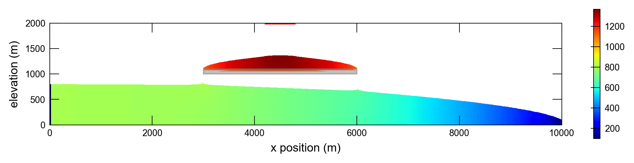
Plotting concentrations...
Plotting conc 1
Plotting conc 2
Plotting conc 3
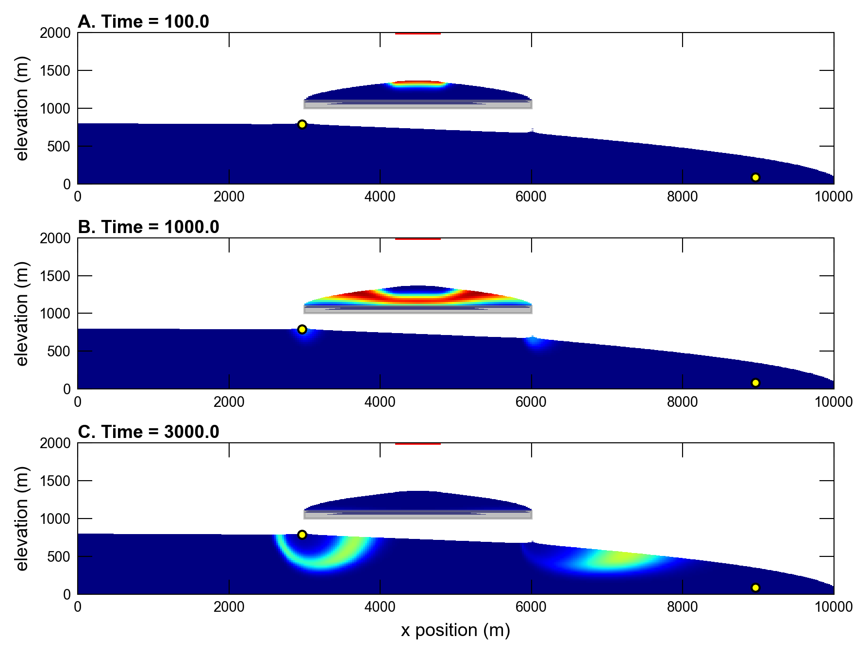
Plotting particle tracks...
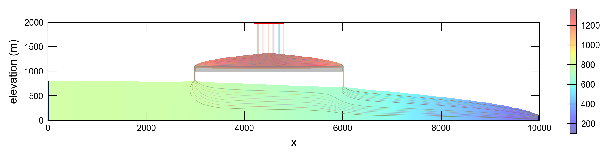
Plotting cvt model results...
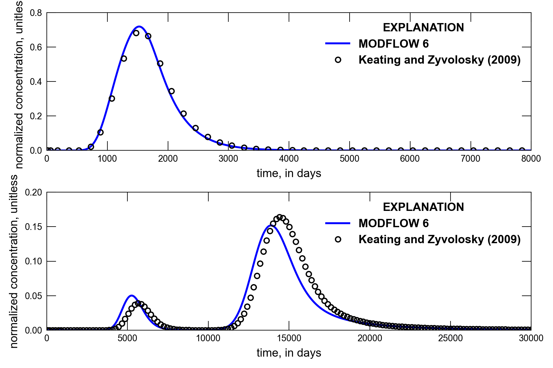
Animating concentrations...