This page was generated from
ex-gwt-gwtgwt-p10.py.
It's also available as a notebook.
MT3DMS Problem 10, Two Domains
The purpose of this example is to demonstrate the model setup for a coupled GWF-GWT simulation with submodels. It replicates the three-dimensional field case study model from the 1999 MT3DMS report. The results are checked for equivalence with the MODFLOW 6 GWT solutions as produced by the example ‘MT3DMS problem 10’.
Initial setup
Import dependencies, define the example name and workspace, and read settings from environment variables.
[1]:
from pathlib import Path

import flopy
import git
import matplotlib.pyplot as plt
import numpy as np
import pooch
from flopy.plot.styles import styles
from flopy.utils.util_array import read1d
from modflow_devtools.misc import get_env

# Example name and workspace paths. If this example is running
# in the git repository, use the folder structure described in
# the README. Otherwise just use the current working directory.
sim_name = "ex-gwt-gwtgwt-p10"
try:
    root = Path(git.Repo(".", search_parent_directories=True).working_dir)
except:
    root = None
workspace = root / "examples" if root else Path.cwd()
figs_path = root / "figures" if root else Path.cwd()
data_path = root / "data" / sim_name if root else Path.cwd()

# Settings from environment variables
write = get_env("WRITE", True)
run = get_env("RUN", True)
plot = get_env("PLOT", True)
plot_show = get_env("PLOT_SHOW", True)
plot_save = get_env("PLOT_SAVE", True)
Define parameters
Define model units, parameters and other settings. Note: the (relative) dimensions of the two models are not configurable.
[2]:
# Model units
length_units = "feet"
time_units = "days"

# Model parameters
nlay = 4  # Number of layers
nlay_inn = 4  # Number of layers
nrow = 61  # Number of rows
nrow_inn = 45  # Number of rows inner model
ncol = 40  # Number of columns
ncol_inn = 28  # Number of columns inner model
delr = "varies"  # Column width ($ft$)
delr_inn = 50  # Column width inner model ($ft$)
delc = "varies"  # Row width ($ft$)
delc_inn = 50  # Row width inner model ($ft$)
xshift = 5100.0  # X offset inner model
yshift = 9100.0  # Y offset inner model
delz = 25.0  # Layer thickness ($ft$)
top = 780.0  # Top of the model ($ft$)
satthk = 100.0  # Saturated thickness ($ft$)
k1 = 60.0  # Horiz. hyd. conductivity of layers 1 and 2 ($ft/day$)
k2 = 520.0  # Horiz. hyd. conductivity of layers 3 and 4 ($ft/day$)
vka = 0.1  # Ratio of vertical to horizontal hydraulic conductivity
rech = 5.0  # Recharge rate ($in/yr$)
crech = 0.0  # Concentration of recharge ($ppm$)
prsity = 0.3  # Porosity
al = 10.0  # Longitudinal dispersivity ($ft$)
trpt = 0.2  # Ratio of horizontal transverse dispersivity to longitudinal dispersivity
trpv = 0.2  # Ratio of vertical transverse dispersivity to longitudinal dispersivity
rhob = 1.7  # Aquifer bulk density ($g/cm^3$)
sp1 = 0.176  # Distribution coefficient ($cm^3/g$)

# Time discretization parameters
perlen = 1000.0  # Simulation time ($days$)
nstp = 500  # Number of time steps
ttsmult = 1.0  # multiplier

# Additional model input
delr = [2000, 1600, 800, 400, 200, 100] + 28 * [50] + [100, 200, 400, 800, 1600, 2000]
delc = (
    [2000, 2000, 2000, 1600, 800, 400, 200, 100]
    + 45 * [50]
    + [100, 200, 400, 800, 1600, 2000, 2000, 2000]
)

hk = [k1, k1, k2, k2]
laytyp = icelltype = 0

# Starting heads from file:
gwt_mt3dms_sim_name = "ex-gwt-mt3dms-p10"
gwt_mt3dms_data_path = data_path.parent / gwt_mt3dms_sim_name if root else Path.cwd()
fname = "p10shead.dat"
fpath = pooch.retrieve(
    url=f"https://github.com/MODFLOW-ORG/modflow6-examples/raw/master/data/{gwt_mt3dms_sim_name}/{fname}",
    fname=fname,
    path=gwt_mt3dms_data_path,
    known_hash="md5:c6591c3c3cfd023ab930b7b1121bfccf",
)
with open(fpath) as f:
    s0 = np.empty((nrow * ncol), dtype=float)
    s0 = read1d(f, s0).reshape((nrow, ncol))
strt = np.zeros((nlay, nrow, ncol), dtype=float)
for k in range(nlay):
    strt[k] = s0
strt_inn = strt[:, 8:53, 6:34]

# Active model domain
idomain = np.ones((nlay, nrow, ncol), dtype=int)
idomain[:, 8:53, 6:34] = 0
idomain_inn = 1
icbund = idomain

# Boundary conditions
rech = 12.7 / 365 / 30.48  # cm/yr -> ft/day
crch = 0.0

# MF6 pumping information for inner DIS
welspd_mf6 = []
#                 [(layer, row, column),     flow, conc]
welspd_mf6.append([(3 - 1, 3 - 1, 23 - 1), -19230.0, 0.00])
welspd_mf6.append([(3 - 1, 11 - 1, 20 - 1), -19230.0, 0.00])
welspd_mf6.append([(3 - 1, 18 - 1, 17 - 1), -19230.0, 0.00])
welspd_mf6.append([(3 - 1, 25 - 1, 14 - 1), -19230.0, 0.00])
welspd_mf6.append([(3 - 1, 32 - 1, 11 - 1), -19230.0, 0.00])
welspd_mf6.append([(3 - 1, 40 - 1, 8 - 1), -19230.0, 0.00])
welspd_mf6.append([(3 - 1, 40 - 1, 3 - 1), -15384.0, 0.00])
welspd_mf6.append([(3 - 1, 44 - 1, 11 - 1), -17307.0, 0.00])
wel_mf6_spd = {0: welspd_mf6}

# Transport related
# Starting concentrations from file:
fname = "p10cinit.dat"
fpath = pooch.retrieve(
    url=f"https://github.com/MODFLOW-ORG/modflow6-examples/raw/master/data/{gwt_mt3dms_sim_name}/{fname}",
    fname=fname,
    path=gwt_mt3dms_data_path,
    known_hash="md5:8e2d3ba7af1ec65bb07f6039d1dfb2c8",
)
with open(fpath) as f:
    c0 = np.empty((nrow * ncol), dtype=float)
    c0 = read1d(f, c0).reshape((nrow, ncol))
sconc = np.zeros((nlay, nrow, ncol), dtype=float)
sconc[1] = 0.2 * c0
sconc[2] = c0

# starting concentration for inner model
sconc_inn = sconc[:, 8:53, 6:34]

# Dispersion
ath1 = al * trpt
atv = al * trpv
dmcoef = 0.0  # ft^2/day

c0 = 0.0
botm = [top - delz * k for k in range(1, nlay + 1)]
mixelm = 0

# Reactive transport related terms
isothm = 1  # sorption type; 1=linear isotherm (equilibrium controlled)
sp2 = 0.0  # w/ isothm = 1 this is read but not used
# ***Note:  In the original documentation for this problem, the following two
#           values are specified in units of g/cm^3 and cm^3/g, respectively.
#           All other units in this problem appear to use ft, including the
#           grid discretization, aquifer K (ft/day), recharge (ft/yr),
#           pumping (ft^3/day), & dispersion (ft).  Because this problem
#           attempts to recreate the original problem for comparison purposes,
#           we are sticking with these values while also acknowledging this
#           discrepancy.
rhob = 1.7  # g/cm^3
sp1 = 0.176  # cm^3/g  (Kd: "Distribution coefficient")

# Transport observations
# Instantiate the basic transport package for the inner model
obs = [
    [3 - 1, 3 - 1, 23 - 1],
    [3 - 1, 11 - 1, 20 - 1],
    [3 - 1, 18 - 1, 17 - 1],
    [3 - 1, 25 - 1, 14 - 1],
    [3 - 1, 32 - 1, 11 - 1],
    [3 - 1, 40 - 1, 8 - 1],
    [3 - 1, 40 - 1, 3 - 1],
    [3 - 1, 44 - 1, 11 - 1],
]

# Solver settings
nouter, ninner = 100, 300
hclose, rclose, relax = 1e-6, 1e-6, 1.0
hclose_gwt, rclose_gwt = 1e-6, 1e-6
percel = 1.0  # HMOC parameters
itrack = 2
wd = 0.5
dceps = 1.0e-5
nplane = 0
npl = 0
nph = 16
npmin = 2
npmax = 32
dchmoc = 1.0e-3
nlsink = nplane
npsink = nph
nadvfd = 1

# Model names
gwfname_out = "gwf-outer"
gwfname_inn = "gwf-inner"
gwtname_out = "gwt-outer"
gwtname_inn = "gwt-inner"

# Exchange data for GWF-GWF and GWT-GWT
exgdata = None

# Advection
scheme = "Undefined"
Model setup
Define functions to build models, write input files, and run the simulation.
[3]:
def build_models():
    sim_ws = workspace / sim_name
    sim = flopy.mf6.MFSimulation(sim_name=sim_name, sim_ws=sim_ws, exe_name="mf6")

    # Instantiating time discretization
    tdis_rc = [(perlen, nstp, 1.0)]
    flopy.mf6.ModflowTdis(sim, nper=1, perioddata=tdis_rc, time_units=time_units)

    # add both solutions to the simulation
    add_flow(sim)
    add_transport(sim)

    # add flow-transport coupling
    flopy.mf6.ModflowGwfgwt(
        sim,
        exgtype="GWF6-GWT6",
        exgmnamea=gwfname_out,
        exgmnameb=gwtname_out,
        filename="outer.gwfgwt",
    )
    flopy.mf6.ModflowGwfgwt(
        sim,
        exgtype="GWF6-GWT6",
        exgmnamea=gwfname_inn,
        exgmnameb=gwtname_inn,
        filename="inner.gwfgwt",
    )

    return sim


def add_flow(sim):
    global exgdata

    # Instantiating solver for flow model
    imsgwf = flopy.mf6.ModflowIms(
        sim,
        print_option="SUMMARY",
        outer_dvclose=hclose,
        outer_maximum=nouter,
        under_relaxation="NONE",
        inner_maximum=ninner,
        inner_dvclose=hclose,
        rcloserecord=rclose,
        linear_acceleration="CG",
        scaling_method="NONE",
        reordering_method="NONE",
        relaxation_factor=relax,
        filename="gwfsolver.ims",
    )

    gwf_outer = add_outer_gwfmodel(sim)
    gwf_inner = add_inner_gwfmodel(sim)

    sim.register_ims_package(imsgwf, [gwf_outer.name, gwf_inner.name])

    # LGR
    exgdata = []
    # east
    for ilay in range(nlay):
        for irow in range(nrow_inn):
            irow_outer = irow + 8
            exgdata.append(
                ((ilay, irow_outer, 5), (ilay, irow, 0), 1, 50.0, 25.0, 50.0, 0.0, 75.0)
            )
    # west
    for ilay in range(nlay):
        for irow in range(nrow_inn):
            irow_outer = irow + 8
            exgdata.append(
                (
                    (ilay, irow_outer, ncol - 6),
                    (ilay, irow, ncol_inn - 1),
                    1,
                    50.0,
                    25.0,
                    50.0,
                    180.0,
                    75.0,
                )
            )
    # north
    for ilay in range(nlay):
        for icol in range(ncol_inn):
            icol_outer = icol + 6
            exgdata.append(
                (
                    (ilay, 7, icol_outer),
                    (ilay, 0, icol),
                    1,
                    50.0,
                    25.0,
                    50.0,
                    270.0,
                    75.0,
                )
            )
    # south
    for ilay in range(nlay):
        for icol in range(ncol_inn):
            icol_outer = icol + 6
            exgdata.append(
                (
                    (ilay, nrow - 8, icol_outer),
                    (ilay, nrow_inn - 1, icol),
                    1,
                    50.0,
                    25.0,
                    50.0,
                    90.0,
                    75.0,
                )
            )

    gwfgwf = flopy.mf6.ModflowGwfgwf(
        sim,
        exgtype="GWF6-GWF6",
        nexg=len(exgdata),
        exgmnamea=gwf_outer.name,
        exgmnameb=gwf_inner.name,
        exchangedata=exgdata,
        xt3d=False,
        print_flows=True,
        auxiliary=["ANGLDEGX", "CDIST"],
        # dev_interfacemodel_on=True,
    )

    # Observe flow for exchange 439
    gwfgwfobs = {}
    gwfgwfobs["gwfgwf.output.obs.csv"] = [
        ["exchange439", "FLOW-JA-FACE", (439 - 1,)],
    ]
    fname = "gwfgwf.input.obs"
    # cdl -- turn off for now as it causes a flopy load fail
    # gwfgwf.obs.initialize(
    #    filename=fname, digits=25, print_input=True, continuous=gwfgwfobs
    # )


def add_outer_gwfmodel(sim):
    """Create the outer GWF model"""
    mname = gwfname_out

    # Instantiating groundwater flow model
    gwf = flopy.mf6.ModflowGwf(
        sim,
        modelname=mname,
        save_flows=True,
        model_nam_file=f"{mname}.nam",
    )

    # Instantiating discretization package
    flopy.mf6.ModflowGwfdis(
        gwf,
        length_units=length_units,
        nlay=nlay,
        nrow=nrow,
        ncol=ncol,
        delr=delr,
        delc=delc,
        top=top,
        botm=botm,
        idomain=idomain,
        filename=f"{mname}.dis",
    )

    # Instantiating initial conditions package for flow model
    flopy.mf6.ModflowGwfic(gwf, strt=strt, filename=f"{mname}.ic")

    # Instantiating node-property flow package
    flopy.mf6.ModflowGwfnpf(
        gwf,
        save_flows=False,
        k33overk=True,
        icelltype=laytyp,
        k=hk,
        k33=vka,
        save_specific_discharge=True,
        filename=f"{mname}.npf",
    )

    # Instantiate storage package
    flopy.mf6.ModflowGwfsto(gwf, ss=0, sy=0, filename=f"{mname}.sto")

    # Instantiating constant head package
    # MF6 constant head boundaries:
    chdspd = []
    # Loop through the left & right sides for all layers.
    # These boundaries are imposed on the outer model.
    for k in np.arange(nlay):
        for i in np.arange(nrow):
            #              (l, r, c),    head,      conc
            chdspd.append([(k, i, 0), strt[k, i, 0], 0.0])  # left
            chdspd.append([(k, i, ncol - 1), strt[k, i, ncol - 1], 0.0])  # right

        for j in np.arange(1, ncol - 1):  # skip corners, already added above
            #              (l, r, c),   head,        conc
            chdspd.append([(k, 0, j), strt[k, 0, j], 0.0])  # top
            chdspd.append([(k, nrow - 1, j), strt[k, nrow - 1, j], 0.0])  # bottom

    chdspd = {0: chdspd}

    flopy.mf6.ModflowGwfchd(
        gwf,
        maxbound=len(chdspd),
        stress_period_data=chdspd,
        save_flows=False,
        auxiliary="CONCENTRATION",
        pname="CHD-1",
        filename=f"{mname}.chd",
    )

    # Instantiate recharge package
    flopy.mf6.ModflowGwfrcha(
        gwf,
        print_flows=True,
        recharge=rech,
        pname="RCH-1",
        filename=f"{mname}.rch",
    )

    # Instantiating output control package for flow model
    flopy.mf6.ModflowGwfoc(
        gwf,
        head_filerecord=f"{mname}.hds",
        budget_filerecord=f"{mname}.bud",
        headprintrecord=[("COLUMNS", 10, "WIDTH", 15, "DIGITS", 6, "GENERAL")],
        saverecord=[
            ("HEAD", "LAST"),
            ("HEAD", "STEPS", "1", "250", "375", "500"),
            ("BUDGET", "LAST"),
        ],
        printrecord=[
            ("HEAD", "LAST"),
            ("BUDGET", "FIRST"),
            ("BUDGET", "LAST"),
        ],
    )

    return gwf


def add_inner_gwfmodel(sim):
    """Create the inner GWF model"""
    mname = gwfname_inn

    # Instantiating groundwater flow submodel
    gwf = flopy.mf6.ModflowGwf(
        sim,
        modelname=mname,
        save_flows=True,
        model_nam_file=f"{mname}.nam",
    )

    # Instantiating discretization package
    flopy.mf6.ModflowGwfdis(
        gwf,
        length_units=length_units,
        nlay=nlay_inn,
        nrow=nrow_inn,
        ncol=ncol_inn,
        delr=delr_inn,
        delc=delc_inn,
        top=top,
        botm=botm,
        idomain=idomain_inn,
        xorigin=xshift,
        yorigin=yshift,
        filename=f"{mname}.dis",
    )

    # Instantiating initial conditions package for flow model
    flopy.mf6.ModflowGwfic(gwf, strt=strt_inn, filename=f"{mname}.ic")

    # Instantiating node-property flow package
    flopy.mf6.ModflowGwfnpf(
        gwf,
        save_flows=False,
        k33overk=True,
        icelltype=laytyp,
        k=hk,
        k33=vka,
        save_specific_discharge=True,
        filename=f"{mname}.npf",
    )

    # Instantiate storage package
    flopy.mf6.ModflowGwfsto(gwf, ss=0, sy=0, filename=f"{mname}.sto")

    # Instantiate recharge package
    flopy.mf6.ModflowGwfrcha(
        gwf,
        print_flows=True,
        recharge=rech,
        pname="RCH-1",
        filename=f"{mname}.rch",
    )

    # Instantiate the wel package
    flopy.mf6.ModflowGwfwel(
        gwf,
        print_input=True,
        print_flows=True,
        stress_period_data=wel_mf6_spd,
        save_flows=False,
        auxiliary="CONCENTRATION",
        pname="WEL-1",
        filename=f"{mname}.wel",
    )

    # Instantiating output control package for flow model
    flopy.mf6.ModflowGwfoc(
        gwf,
        head_filerecord=f"{mname}.hds",
        budget_filerecord=f"{mname}.bud",
        headprintrecord=[("COLUMNS", 10, "WIDTH", 15, "DIGITS", 6, "GENERAL")],
        saverecord=[
            ("HEAD", "LAST"),
            ("HEAD", "STEPS", "1", "250", "375", "500"),
            ("BUDGET", "LAST"),
        ],
        printrecord=[
            ("HEAD", "LAST"),
            ("BUDGET", "FIRST"),
            ("BUDGET", "LAST"),
        ],
    )

    return gwf


def add_transport(sim):
    """Add the transport models and exchange to the simulation"""
    # Create iterative model solution
    imsgwt = flopy.mf6.ModflowIms(
        sim,
        print_option="SUMMARY",
        outer_dvclose=hclose_gwt,
        outer_maximum=nouter,
        under_relaxation="NONE",
        inner_maximum=ninner,
        inner_dvclose=hclose_gwt,
        rcloserecord=rclose_gwt,
        linear_acceleration="BICGSTAB",
        scaling_method="NONE",
        reordering_method="NONE",
        relaxation_factor=relax,
        filename="gwtsolver.ims",
    )

    # Instantiating transport advection package
    global scheme
    if mixelm >= 0:
        scheme = "UPSTREAM"
    elif mixelm == -1:
        scheme = "TVD"
    else:
        raise Exception()

    # Add transport models
    gwt_outer = add_outer_gwtmodel(sim)
    gwt_inner = add_inner_gwtmodel(sim)

    sim.register_ims_package(imsgwt, [gwt_outer.name, gwt_inner.name])

    # Create transport-transport coupling
    assert exgdata is not None
    gwtgwt = flopy.mf6.ModflowGwtgwt(
        sim,
        exgtype="GWT6-GWT6",
        gwfmodelname1=gwfname_out,
        gwfmodelname2=gwfname_inn,
        adv_scheme=scheme,
        nexg=len(exgdata),
        exgmnamea=gwt_outer.name,
        exgmnameb=gwt_inner.name,
        exchangedata=exgdata,
        auxiliary=["ANGLDEGX", "CDIST"],
    )

    # Observe mass flow for exchange 439
    gwtgwtobs = {}
    gwtgwtobs["gwtgwt.output.obs.csv"] = [
        ["exchange439", "FLOW-JA-FACE", (439 - 1,)],
    ]
    fname = "gwtgwt.input.obs"
    # cdl -- turn off for now as it causes a flopy load fail
    # gwtgwt.obs.initialize(
    #    filename=fname, digits=25, print_input=True, continuous=gwtgwtobs
    # )

    return sim


def add_outer_gwtmodel(sim):
    """Create the outer GWT model"""
    mname = gwtname_out
    gwt = flopy.mf6.MFModel(
        sim,
        model_type="gwt6",
        modelname=mname,
        model_nam_file=f"{mname}.nam",
    )
    gwt.name_file.save_flows = True

    # Instantiating transport discretization package
    flopy.mf6.ModflowGwtdis(
        gwt,
        nlay=nlay,
        nrow=nrow,
        ncol=ncol,
        delr=delr,
        delc=delc,
        top=top,
        botm=botm,
        idomain=idomain,
        filename=f"{mname}.dis",
    )

    # Instantiating transport initial concentrations
    flopy.mf6.ModflowGwtic(gwt, strt=sconc, filename=f"{mname}.ic")

    flopy.mf6.ModflowGwtadv(gwt, scheme=scheme, filename=f"{mname}.adv")

    # Instantiating transport dispersion package
    if al != 0:
        flopy.mf6.ModflowGwtdsp(
            gwt,
            alh=al,
            ath1=ath1,
            atv=atv,
            pname="DSP-1",
            filename=f"{mname}.dsp",
        )

    # Instantiating transport mass storage package
    kd = sp1
    flopy.mf6.ModflowGwtmst(
        gwt,
        porosity=prsity,
        first_order_decay=False,
        decay=None,
        decay_sorbed=None,
        sorption="linear",
        bulk_density=rhob,
        distcoef=kd,
        pname="MST-1",
        filename=f"{mname}.mst",
    )

    # Instantiating transport source-sink mixing package
    sourcerecarray = [("CHD-1", "AUX", "CONCENTRATION")]
    flopy.mf6.ModflowGwtssm(
        gwt,
        sources=sourcerecarray,
        print_flows=True,
        filename=f"{mname}.ssm",
    )

    # Instantiating transport output control package
    flopy.mf6.ModflowGwtoc(
        gwt,
        budget_filerecord=f"{mname}.cbc",
        concentration_filerecord=f"{mname}.ucn",
        concentrationprintrecord=[("COLUMNS", 10, "WIDTH", 15, "DIGITS", 6, "GENERAL")],
        saverecord=[
            ("CONCENTRATION", "LAST"),
            ("CONCENTRATION", "STEPS", "1", "250", "375", "500"),
            ("BUDGET", "LAST"),
        ],
        printrecord=[("CONCENTRATION", "LAST"), ("BUDGET", "LAST")],
        filename=f"{mname}.oc",
    )

    return gwt


def add_inner_gwtmodel(sim):
    """Create the inner GWT model"""
    mname = gwtname_inn
    gwt = flopy.mf6.MFModel(
        sim,
        model_type="gwt6",
        modelname=mname,
        model_nam_file=f"{mname}.nam",
    )
    gwt.name_file.save_flows = True

    # Instantiating transport discretization package
    flopy.mf6.ModflowGwtdis(
        gwt,
        nlay=nlay_inn,
        nrow=nrow_inn,
        ncol=ncol_inn,
        delr=delr_inn,
        delc=delc_inn,
        top=top,
        botm=botm,
        idomain=idomain_inn,
        xorigin=xshift,
        yorigin=yshift,
        filename=f"{mname}.dis",
    )

    # Instantiating transport initial concentrations
    flopy.mf6.ModflowGwtic(gwt, strt=sconc_inn, filename=f"{mname}.ic")

    flopy.mf6.ModflowGwtadv(gwt, scheme=scheme, filename=f"{mname}.adv")

    # Instantiating transport dispersion package
    if al != 0:
        flopy.mf6.ModflowGwtdsp(
            gwt,
            alh=al,
            ath1=ath1,
            atv=atv,
            pname="DSP-1",
            filename=f"{mname}.dsp",
        )

    # Instantiating transport mass storage package
    kd = sp1
    flopy.mf6.ModflowGwtmst(
        gwt,
        porosity=prsity,
        first_order_decay=False,
        decay=None,
        decay_sorbed=None,
        sorption="linear",
        bulk_density=rhob,
        distcoef=kd,
        pname="MST-1",
        filename=f"{mname}.mst",
    )

    # Instantiating transport source-sink mixing package
    sourcerecarray = None
    flopy.mf6.ModflowGwtssm(
        gwt,
        sources=sourcerecarray,
        print_flows=True,
        filename=f"{mname}.ssm",
    )

    # Instantiating transport output control package
    flopy.mf6.ModflowGwtoc(
        gwt,
        budget_filerecord=f"{mname}.cbc",
        concentration_filerecord=f"{mname}.ucn",
        concentrationprintrecord=[("COLUMNS", 10, "WIDTH", 15, "DIGITS", 6, "GENERAL")],
        saverecord=[
            ("CONCENTRATION", "LAST"),
            ("CONCENTRATION", "STEPS", "1", "250", "375", "500"),
            ("BUDGET", "LAST"),
        ],
        printrecord=[("CONCENTRATION", "LAST"), ("BUDGET", "LAST")],
        filename=f"{mname}.oc",
    )

    return gwt


def run_models(sim):
    success = True
    if run:
        success, buff = sim.run_simulation()
        if not success:
            print(buff)
    return success
Plotting results
Define functions to plot model results.
[4]:
# Figure properties
figure_size = (6, 8)
# Load MODFLOW 6 reference for the concentrations (GWT MT3DMS p10)
def get_reference_data_conc():
fname = "gwt-p10-mf6_conc_lay3_1days.txt"
fpath = pooch.retrieve(
url=f"https://github.com/MODFLOW-ORG/modflow6-examples/raw/master/data/{sim_name}/{fname}",
fname=fname,
path=data_path,
known_hash="md5:bbb596110559d00b7f01032998cf35f4",
)
conc1 = np.loadtxt(fpath)
fname = "gwt-p10-mf6_conc_lay3_500days.txt"
fpath = pooch.retrieve(
url=f"https://github.com/MODFLOW-ORG/modflow6-examples/raw/master/data/{sim_name}/{fname}",
fname=fname,
path=data_path,
known_hash="md5:3b3b9321ae6c801fec7d3562aa44a009",
)
conc500 = np.loadtxt(fpath)
fname = "gwt-p10-mf6_conc_lay3_750days.txt"
fpath = pooch.retrieve(
url=f"https://github.com/MODFLOW-ORG/modflow6-examples/raw/master/data/{sim_name}/{fname}",
fname=fname,
path=data_path,
known_hash="md5:0d1c2e7682a946e11b56f87c28c0ebd7",
)
conc750 = np.loadtxt(fpath)
fname = "gwt-p10-mf6_conc_lay3_1000days.txt"
fpath = pooch.retrieve(
url=f"https://github.com/MODFLOW-ORG/modflow6-examples/raw/master/data/{sim_name}/{fname}",
fname=fname,
path=data_path,
known_hash="md5:c5fe612424e5f83fb2ac46cd4fdc8fb6",
)
conc1000 = np.loadtxt(fpath)
return [conc1, conc500, conc750, conc1000]
# Load MODFLOW 6 reference for heads (GWT MT3DMS p10)
def get_reference_data_heads():
fname = "gwt-p10-mf6_head_lay3_1days.txt"
fpath = pooch.retrieve(
url=f"https://github.com/MODFLOW-ORG/modflow6-examples/raw/master/data/{sim_name}/{fname}",
fname=fname,
path=data_path,
known_hash="md5:0c5ce894877692b0a018587a2df068d6",
)
head1 = np.loadtxt(fpath)
fname = "gwt-p10-mf6_head_lay3_500days.txt"
fpath = pooch.retrieve(
url=f"https://github.com/MODFLOW-ORG/modflow6-examples/raw/master/data/{sim_name}/{fname}",
fname=fname,
path=data_path,
known_hash="md5:b4b56f9ecad0abafc6c62072cc5f15e9",
)
head500 = np.loadtxt(fpath)
fname = "gwt-p10-mf6_head_lay3_750days.txt"
fpath = pooch.retrieve(
url=f"https://github.com/MODFLOW-ORG/modflow6-examples/raw/master/data/{sim_name}/{fname}",
fname=fname,
path=data_path,
known_hash="md5:1c35fee2f7764c1c28eb84ed98b1300c",
)
head750 = np.loadtxt(fpath)
fname = "gwt-p10-mf6_head_lay3_1000days.txt"
fpath = pooch.retrieve(
url=f"https://github.com/MODFLOW-ORG/modflow6-examples/raw/master/data/{sim_name}/{fname}",
fname=fname,
path=data_path,
known_hash="md5:b8e67997ca429f6f20e15852fb2fba9f",
)
head1000 = np.loadtxt(fpath)
return [head1, head500, head750, head1000]
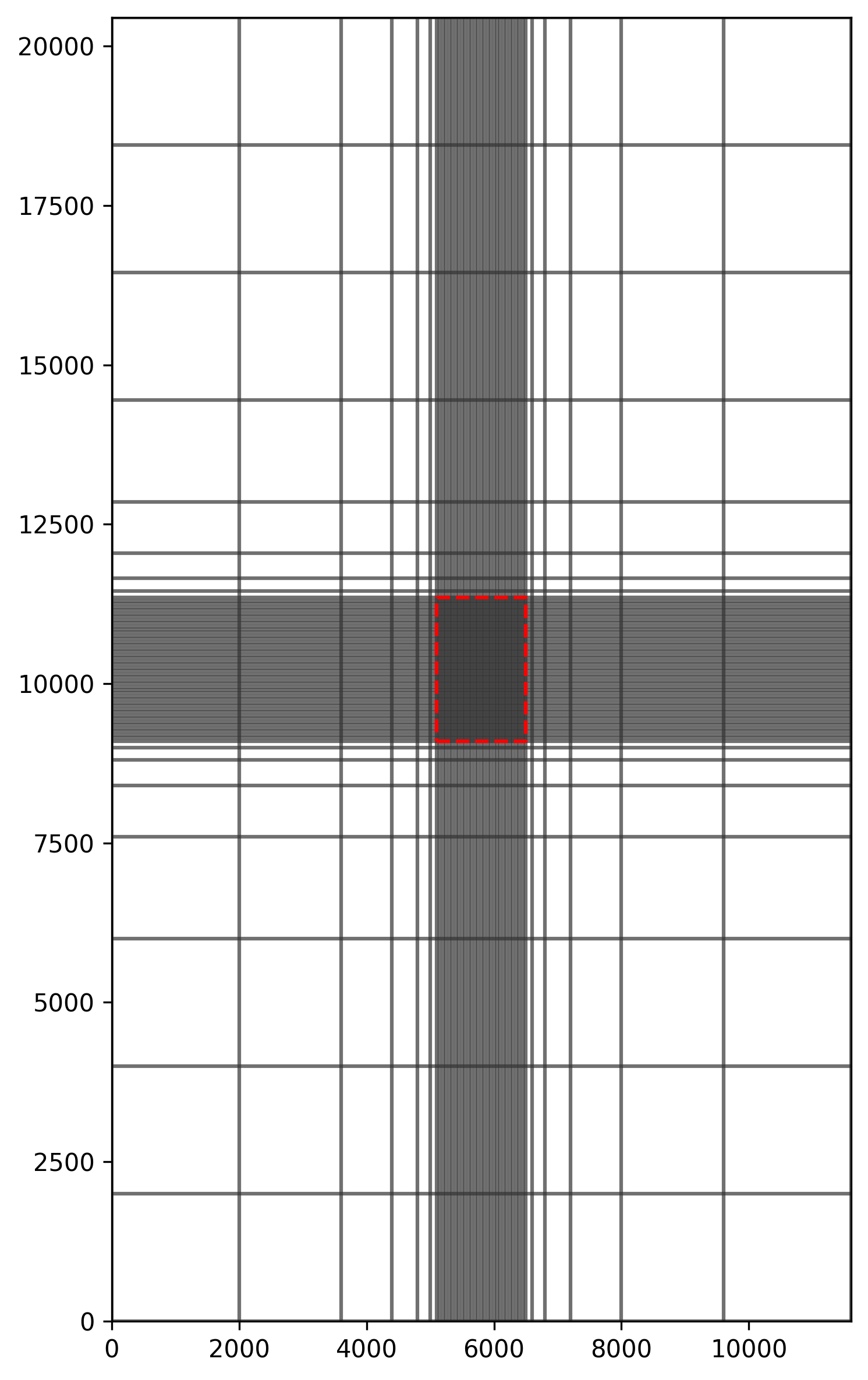
# Plot the inner and outer grid
def plot_grids(sim):
xmin = xshift
ymin = yshift
xmax = xshift + 1400
ymax = yshift + 2250
fig = plt.figure(figsize=figure_size, dpi=300, tight_layout=True)
ax = fig.add_subplot(1, 1, 1, aspect="equal")
gwt_outer = sim.get_model(gwtname_out)
mm = flopy.plot.PlotMapView(model=gwt_outer)
mm.plot_grid(color="0.2", alpha=0.7)
ax.plot([xmin, xmax, xmax, xmin, xmin], [ymin, ymin, ymax, ymax, ymin], "r--")
fpath = figs_path / "ex-gwtgwt-p10-modelgrid.png"
fig.savefig(fpath)
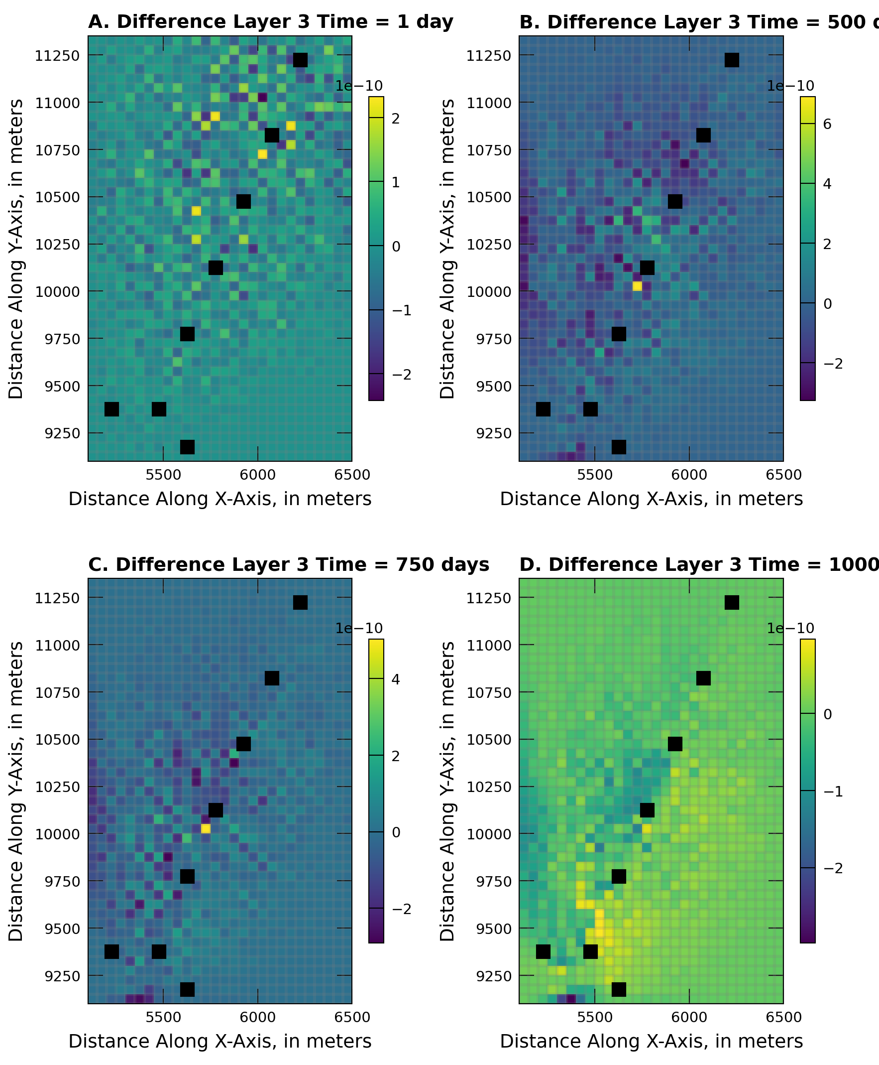
# Plot the difference in concentration after 1,500,750,1000 days
# between this coupled model setup using a GWT-GWT exchange and the
# single model reference
def plot_difference_conc(sim):
conc_singlemodel_lay3 = get_reference_data_conc()
# Get the concentration output
gwt_outer = sim.get_model(gwtname_out)
gwt = sim.get_model(gwtname_inn)
ucnobj_mf6 = gwt.output.concentration()
conc_mf6 = ucnobj_mf6.get_alldata()
ucnobj_mf6_outer = gwt_outer.output.concentration()
conc_mf6_outer = ucnobj_mf6_outer.get_alldata()
# Create figure for scenario
with styles.USGSPlot():
plt.rcParams["lines.dashed_pattern"] = [5.0, 5.0]
fig = plt.figure(figsize=figure_size, dpi=300, tight_layout=True)
# Difference in concentration @ 1 day
ax = fig.add_subplot(2, 2, 1, aspect="equal")
mm = flopy.plot.PlotMapView(model=gwt_outer)
mm.plot_grid(color=".5", alpha=0.2)
istep = 0
ilayer = 2
c_1day = conc_mf6_outer[istep]
c_1day[:, 8:53, 6:34] = conc_mf6[istep]
c_1day_singlemodel_lay3 = conc_singlemodel_lay3[istep]
pa = mm.plot_array(c_1day[ilayer] - c_1day_singlemodel_lay3)
xc, yc = gwt.modelgrid.xycenters
plt.xlim(5100, 5100 + 28 * 50)
plt.ylim(9100, 9100 + 45 * 50)
plt.xlabel("Distance Along X-Axis, in meters")
plt.ylabel("Distance Along Y-Axis, in meters")
plt.colorbar(pa, shrink=0.5)
# Plot the wells as well
for cid, f, c in welspd_mf6:
plt.plot(xshift + xc[cid[2]], yshift + yc[cid[1]], "ks")
title = "Difference Layer 3 Time = 1 day"
styles.heading(letter="A", heading=title)
# Difference in concentration @ 500 days
ax = fig.add_subplot(2, 2, 2, aspect="equal")
mm = flopy.plot.PlotMapView(model=gwt_outer)
mm.plot_grid(color=".5", alpha=0.2)
istep = 1
ilayer = 2
c_500days = conc_mf6_outer[istep]
c_500days[:, 8:53, 6:34] = conc_mf6[istep]
c_500days_singlemodel_lay3 = conc_singlemodel_lay3[istep]
pa = mm.plot_array(c_500days[ilayer] - c_500days_singlemodel_lay3)
plt.xlim(5100, 5100 + 28 * 50)
plt.ylim(9100, 9100 + 45 * 50)
plt.xlabel("Distance Along X-Axis, in meters")
plt.ylabel("Distance Along Y-Axis, in meters")
plt.colorbar(pa, shrink=0.5)
for cid, f, c in welspd_mf6:
plt.plot(xshift + xc[cid[2]], yshift + yc[cid[1]], "ks")
title = "Difference Layer 3 Time = 500 days"
styles.heading(letter="B", heading=title)
# Difference in concentration @ 750 days
ax = fig.add_subplot(2, 2, 3, aspect="equal")
mm = flopy.plot.PlotMapView(model=gwt_outer)
mm.plot_grid(color=".5", alpha=0.2)
istep = 2
ilayer = 2
c_750days = conc_mf6_outer[istep]
c_750days[:, 8:53, 6:34] = conc_mf6[istep]
c_750days_singlemodel_lay3 = conc_singlemodel_lay3[istep]
pa = mm.plot_array(c_750days[ilayer] - c_750days_singlemodel_lay3)
plt.xlim(5100, 5100 + 28 * 50)
plt.ylim(9100, 9100 + 45 * 50)
plt.xlabel("Distance Along X-Axis, in meters")
plt.ylabel("Distance Along Y-Axis, in meters")
plt.colorbar(pa, shrink=0.5)
for cid, f, c in welspd_mf6:
plt.plot(xshift + xc[cid[2]], yshift + yc[cid[1]], "ks")
title = "Difference Layer 3 Time = 750 days"
styles.heading(letter="C", heading=title)
# Difference in concentration @ 1000 days
ax = fig.add_subplot(2, 2, 4, aspect="equal")
mm = flopy.plot.PlotMapView(model=gwt_outer)
mm.plot_grid(color=".5", alpha=0.2)
istep = 3
ilayer = 2
c_1000days = conc_mf6_outer[istep]
c_1000days[:, 8:53, 6:34] = conc_mf6[istep]
c_1000days_singlemodel_lay3 = conc_singlemodel_lay3[istep]
pa = mm.plot_array(c_1000days[ilayer] - c_1000days_singlemodel_lay3)
plt.xlim(5100, 5100 + 28 * 50)
plt.ylim(9100, 9100 + 45 * 50)
plt.xlabel("Distance Along X-Axis, in meters")
plt.ylabel("Distance Along Y-Axis, in meters")
plt.colorbar(pa, shrink=0.5)
for cid, f, c in welspd_mf6:
plt.plot(xshift + xc[cid[2]], yshift + yc[cid[1]], "ks")
title = "Difference Layer 3 Time = 1000 days"
styles.heading(letter="D", heading=title)
fpath = figs_path / "ex-gwtgwt-p10-diffconc.png"
fig.savefig(fpath)
# Plot the difference in head after 1,500,750,1000 days
# between this coupled model and the single model reference
def plot_difference_heads(sim):
head_singlemodel_lay3 = get_reference_data_heads()
# Get the concentration output
gwf_outer = sim.get_model(gwfname_out)
gwf = sim.get_model(gwfname_inn)
hobj_mf6 = gwf.output.head()
head_mf6 = hobj_mf6.get_alldata()
hobj_mf6_outer = gwf_outer.output.head()
head_mf6_outer = hobj_mf6_outer.get_alldata()
# Create figure for scenario
with styles.USGSPlot():
plt.rcParams["lines.dashed_pattern"] = [5.0, 5.0]
fig = plt.figure(figsize=figure_size, dpi=300, tight_layout=True)
# Difference in heads @ 1 day
ax = fig.add_subplot(2, 2, 1, aspect="equal")
mm = flopy.plot.PlotMapView(model=gwf_outer)
mm.plot_grid(color=".5", alpha=0.2)
istep = 0
ilayer = 2
h_1day = head_mf6_outer[istep]
h_1day[:, 8:53, 6:34] = head_mf6[istep]
h_1day_singlemodel_lay3 = head_singlemodel_lay3[istep]
pa = mm.plot_array(h_1day[ilayer] - h_1day_singlemodel_lay3)
xc, yc = gwf.modelgrid.xycenters
plt.xlim(5100, 5100 + 28 * 50)
plt.ylim(9100, 9100 + 45 * 50)
plt.xlabel("Distance Along X-Axis, in meters")
plt.ylabel("Distance Along Y-Axis, in meters")
plt.colorbar(pa, shrink=0.5)
# Plot the wells as well
for cid, f, c in welspd_mf6:
plt.plot(xshift + xc[cid[2]], yshift + yc[cid[1]], "ks")
title = "Difference Layer 3 Time = 1 day"
styles.heading(letter="A", heading=title)
# Difference in heads @ 500 days
ax = fig.add_subplot(2, 2, 2, aspect="equal")
mm = flopy.plot.PlotMapView(model=gwf_outer)
mm.plot_grid(color=".5", alpha=0.2)
istep = 1
ilayer = 2
h_500days = head_mf6_outer[istep]
h_500days[:, 8:53, 6:34] = head_mf6[istep]
h_500days_singlemodel_lay3 = head_singlemodel_lay3[istep]
pa = mm.plot_array(h_500days[ilayer] - h_500days_singlemodel_lay3)
plt.xlim(5100, 5100 + 28 * 50)
plt.ylim(9100, 9100 + 45 * 50)
plt.xlabel("Distance Along X-Axis, in meters")
plt.ylabel("Distance Along Y-Axis, in meters")
plt.colorbar(pa, shrink=0.5)
for cid, f, c in welspd_mf6:
plt.plot(xshift + xc[cid[2]], yshift + yc[cid[1]], "ks")
title = "Difference Layer 3 Time = 500 days"
styles.heading(letter="B", heading=title)
# Difference in heads @ 750 days
ax = fig.add_subplot(2, 2, 3, aspect="equal")
mm = flopy.plot.PlotMapView(model=gwf_outer)
mm.plot_grid(color=".5", alpha=0.2)
istep = 2
ilayer = 2
h_750days = head_mf6_outer[istep]
h_750days[:, 8:53, 6:34] = head_mf6[istep]
h_750days_singlemodel_lay3 = head_singlemodel_lay3[istep]
pa = mm.plot_array(h_750days[ilayer] - h_750days_singlemodel_lay3)
plt.xlim(5100, 5100 + 28 * 50)
plt.ylim(9100, 9100 + 45 * 50)
plt.xlabel("Distance Along X-Axis, in meters")
plt.ylabel("Distance Along Y-Axis, in meters")
plt.colorbar(pa, shrink=0.5)
for cid, f, c in welspd_mf6:
plt.plot(xshift + xc[cid[2]], yshift + yc[cid[1]], "ks")
title = "Difference Layer 3 Time = 750 days"
styles.heading(letter="C", heading=title)
# Difference in heads @ 1000 days
ax = fig.add_subplot(2, 2, 4, aspect="equal")
mm = flopy.plot.PlotMapView(model=gwf_outer)
mm.plot_grid(color=".5", alpha=0.2)
istep = 3
ilayer = 2
h_1000days = head_mf6_outer[istep]
h_1000days[:, 8:53, 6:34] = head_mf6[istep]
h_1000days_singlemodel_lay3 = head_singlemodel_lay3[istep]
pa = mm.plot_array(h_1000days[ilayer] - h_1000days_singlemodel_lay3)
plt.xlim(5100, 5100 + 28 * 50)
plt.ylim(9100, 9100 + 45 * 50)
plt.xlabel("Distance Along X-Axis, in meters")
plt.ylabel("Distance Along Y-Axis, in meters")
plt.colorbar(pa, shrink=0.5)
for cid, f, c in welspd_mf6:
plt.plot(xshift + xc[cid[2]], yshift + yc[cid[1]], "ks")
title = "Difference Layer 3 Time = 1000 days"
styles.heading(letter="D", heading=title)
fpath = figs_path / "ex-gwtgwt-p10-diffhead.png"
fig.savefig(fpath)
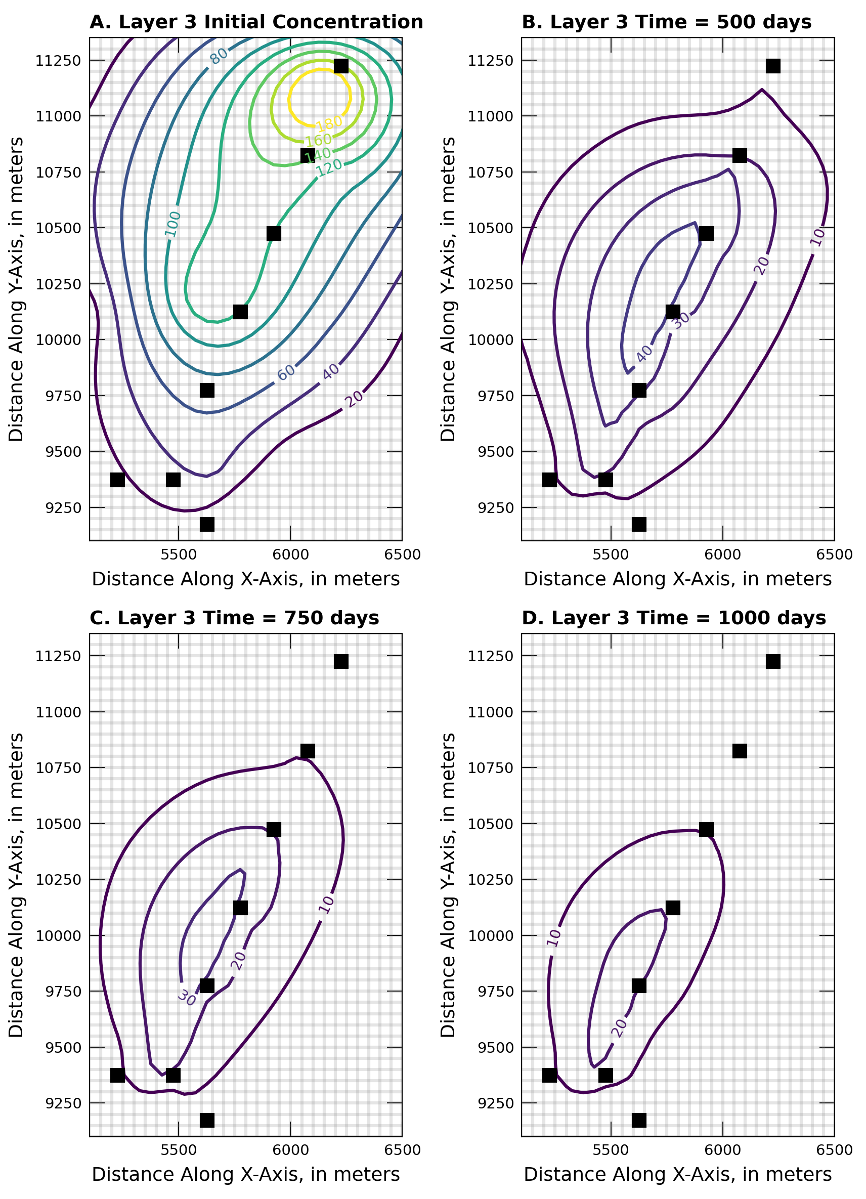
# Plot the concentration, this figure should be compared to the same figure in MT3DMS problem 10
def plot_concentration(sim):
# Get the concentration output
gwt_outer = sim.get_model(gwtname_out)
gwt = sim.get_model(gwtname_inn)
ucnobj_mf6 = gwt.output.concentration()
conc_mf6 = ucnobj_mf6.get_alldata()
ucnobj_mf6_outer = gwt_outer.output.concentration()
conc_mf6_outer = ucnobj_mf6_outer.get_alldata()
# Create figure for scenario
with styles.USGSPlot():
plt.rcParams["lines.dashed_pattern"] = [5.0, 5.0]
xc, yc = gwt.modelgrid.xycenters
# Plot init. concentration (lay=3)
fig = plt.figure(figsize=figure_size, dpi=300, tight_layout=True)
ax = fig.add_subplot(2, 2, 1, aspect="equal")
mm = flopy.plot.PlotMapView(model=gwt_outer)
mm.plot_grid(color=".5", alpha=0.2)
cs = mm.contour_array(sconc[2], levels=np.arange(20, 200, 20))
plt.xlim(5100, 5100 + 28 * 50)
plt.ylim(9100, 9100 + 45 * 50)
plt.xlabel("Distance Along X-Axis, in meters")
plt.ylabel("Distance Along Y-Axis, in meters")
plt.clabel(cs, fmt=r"%3d")
# Plot the wells as well
for cid, f, c in welspd_mf6:
plt.plot(xshift + xc[cid[2]], yshift + yc[cid[1]], "ks")
title = "Layer 3 Initial Concentration"
styles.heading(letter="A", heading=title)
ax = fig.add_subplot(2, 2, 2, aspect="equal")
mm = flopy.plot.PlotMapView(model=gwt_outer)
mm.plot_grid(color=".5", alpha=0.2)
c_500days = conc_mf6_outer[1]
c_500days[:, 8:53, 6:34] = conc_mf6[1] # Concentration @ 500 days
cs = mm.contour_array(c_500days[2], levels=np.arange(10, 200, 10))
plt.xlim(5100, 5100 + 28 * 50)
plt.ylim(9100, 9100 + 45 * 50)
plt.xlabel("Distance Along X-Axis, in meters")
plt.ylabel("Distance Along Y-Axis, in meters")
plt.clabel(cs, fmt=r"%3d")
for cid, f, c in welspd_mf6:
plt.plot(xshift + xc[cid[2]], yshift + yc[cid[1]], "ks")
title = "Layer 3 Time = 500 days"
styles.heading(letter="B", heading=title)
ax = fig.add_subplot(2, 2, 3, aspect="equal")
mm = flopy.plot.PlotMapView(model=gwt_outer)
mm.plot_grid(color=".5", alpha=0.2)
c_750days = conc_mf6_outer[2]
c_750days[:, 8:53, 6:34] = conc_mf6[2] # Concentration @ 750 days
cs = mm.contour_array(c_750days[2], levels=np.arange(10, 200, 10))
plt.xlim(5100, 5100 + 28 * 50)
plt.ylim(9100, 9100 + 45 * 50)
plt.xlabel("Distance Along X-Axis, in meters")
plt.ylabel("Distance Along Y-Axis, in meters")
plt.clabel(cs, fmt=r"%3d")
for cid, f, c in welspd_mf6:
plt.plot(xshift + xc[cid[2]], yshift + yc[cid[1]], "ks")
title = "Layer 3 Time = 750 days"
styles.heading(letter="C", heading=title)
ax = fig.add_subplot(2, 2, 4, aspect="equal")
mm = flopy.plot.PlotMapView(model=gwt_outer)
mm.plot_grid(color=".5", alpha=0.2)
c_1000days = conc_mf6_outer[3]
c_1000days[:, 8:53, 6:34] = conc_mf6[3] # Concentration @ 1000 days
cs = mm.contour_array(c_1000days[2], levels=np.arange(10, 200, 10))
plt.xlim(5100, 5100 + 28 * 50)
plt.ylim(9100, 9100 + 45 * 50)
plt.xlabel("Distance Along X-Axis, in meters")
plt.ylabel("Distance Along Y-Axis, in meters")
plt.clabel(cs, fmt=r"%3d")
for cid, f, c in welspd_mf6:
plt.plot(xshift + xc[cid[2]], yshift + yc[cid[1]], "ks")
title = "Layer 3 Time = 1000 days"
styles.heading(letter="D", heading=title)
fpath = figs_path / "ex-gwtgwt-p10-concentration.png"
fig.savefig(fpath)
# Generates all plots
def plot_results(sim):
print("Plotting model results...")
plot_grids(sim)
plot_concentration(sim)
plot_difference_conc(sim)
plot_difference_heads(sim)
Running the example
Define and invoke a function to run the example scenario, then plot results.
[5]:
def scenario():
    sim = build_models()
    if write:
        sim.write_simulation()
    if run:
        run_models(sim)
    if plot:
        plot_results(sim)


scenario()
writing simulation...
  writing simulation name file...
  writing simulation tdis package...
  writing solution package ims_-1...
  writing solution package ims_0...
  writing package ex-gwt-gwtgwt-p10.gwfgwf...
  writing package ex-gwt-gwtgwt-p10.gwtgwt...
  writing package outer.gwfgwt...
  writing package inner.gwfgwt...
  writing model gwf-outer...
    writing model name file...
    writing package dis...
    writing package ic...
    writing package npf...
    writing package sto...
    writing package chd-1...
INFORMATION: maxbound in ('', 'chd', 'dimensions') changed to 792 based on size of stress_period_data
    writing package rch-1...
    writing package oc...
  writing model gwf-inner...
    writing model name file...
    writing package dis...
    writing package ic...
    writing package npf...
    writing package sto...
    writing package rch-1...
    writing package wel-1...
INFORMATION: maxbound in ('', 'wel', 'dimensions') changed to 8 based on size of stress_period_data
    writing package oc...
  writing model gwt-outer...
    writing model name file...
    writing package dis...
    writing package ic...
    writing package adv...
    writing package dsp-1...
    writing package mst-1...
    writing package ssm...
    writing package oc...
  writing model gwt-inner...
    writing model name file...
    writing package dis...
    writing package ic...
    writing package adv...
    writing package dsp-1...
    writing package mst-1...
    writing package ssm...
    writing package oc...
FloPy is using the following executable to run the model: ../../../../../../.local/bin/modflow/mf6
                                   MODFLOW 6
                U.S. GEOLOGICAL SURVEY MODULAR HYDROLOGIC MODEL
                  VERSION 6.8.0.dev0 (preliminary) 02/06/2026
                               ***DEVELOP MODE***

        MODFLOW 6 compiled Feb 15 2026 14:55:26 with GCC version 13.3.0

This software is preliminary or provisional and is subject to
revision. It is being provided to meet the need for timely best
science. The software has not received final approval by the U.S.
Geological Survey (USGS). No warranty, expressed or implied, is made
by the USGS or the U.S. Government as to the functionality of the
software and related material nor shall the fact of release
constitute any such warranty. The software is provided on the
condition that neither the USGS nor the U.S. Government shall be held
liable for any damages resulting from the authorized or unauthorized
use of the software.


 MODFLOW runs in SEQUENTIAL mode

 Run start date and time (yyyy/mm/dd hh:mm:ss): 2026/02/15 15:02:29

 Writing simulation list file: mfsim.lst
 Using Simulation name file: mfsim.nam
    Solving:  Stress period:     1    Time step:     1
    Solving:  Stress period:     1    Time step:     2
    Solving:  Stress period:     1    Time step:     3
    Solving:  Stress period:     1    Time step:     4
    Solving:  Stress period:     1    Time step:     5
    Solving:  Stress period:     1    Time step:     6
    Solving:  Stress period:     1    Time step:     7
    Solving:  Stress period:     1    Time step:     8
    Solving:  Stress period:     1    Time step:     9
    Solving:  Stress period:     1    Time step:    10
    Solving:  Stress period:     1    Time step:    11
    Solving:  Stress period:     1    Time step:    12
    Solving:  Stress period:     1    Time step:    13
    Solving:  Stress period:     1    Time step:    14
    Solving:  Stress period:     1    Time step:    15
    Solving:  Stress period:     1    Time step:    16
    Solving:  Stress period:     1    Time step:    17
    Solving:  Stress period:     1    Time step:    18
    Solving:  Stress period:     1    Time step:    19
    Solving:  Stress period:     1    Time step:    20
    Solving:  Stress period:     1    Time step:    21
    Solving:  Stress period:     1    Time step:    22
    Solving:  Stress period:     1    Time step:    23
    Solving:  Stress period:     1    Time step:    24
    Solving:  Stress period:     1    Time step:    25
    Solving:  Stress period:     1    Time step:    26
    Solving:  Stress period:     1    Time step:    27
    Solving:  Stress period:     1    Time step:    28
    Solving:  Stress period:     1    Time step:    29
    Solving:  Stress period:     1    Time step:    30
    Solving:  Stress period:     1    Time step:    31
    Solving:  Stress period:     1    Time step:    32
    Solving:  Stress period:     1    Time step:    33
    Solving:  Stress period:     1    Time step:    34
    Solving:  Stress period:     1    Time step:    35
    Solving:  Stress period:     1    Time step:    36
    Solving:  Stress period:     1    Time step:    37
    Solving:  Stress period:     1    Time step:    38
    Solving:  Stress period:     1    Time step:    39
    Solving:  Stress period:     1    Time step:    40
    Solving:  Stress period:     1    Time step:    41
    Solving:  Stress period:     1    Time step:    42
    Solving:  Stress period:     1    Time step:    43
    Solving:  Stress period:     1    Time step:    44
    Solving:  Stress period:     1    Time step:    45
    Solving:  Stress period:     1    Time step:    46
    Solving:  Stress period:     1    Time step:    47
    Solving:  Stress period:     1    Time step:    48
    Solving:  Stress period:     1    Time step:    49
    Solving:  Stress period:     1    Time step:    50
    Solving:  Stress period:     1    Time step:    51
    Solving:  Stress period:     1    Time step:    52
    Solving:  Stress period:     1    Time step:    53
    Solving:  Stress period:     1    Time step:    54
    Solving:  Stress period:     1    Time step:    55
    Solving:  Stress period:     1    Time step:    56
    Solving:  Stress period:     1    Time step:    57
    Solving:  Stress period:     1    Time step:    58
    Solving:  Stress period:     1    Time step:    59
    Solving:  Stress period:     1    Time step:    60
    Solving:  Stress period:     1    Time step:    61
    Solving:  Stress period:     1    Time step:    62
    Solving:  Stress period:     1    Time step:    63
    Solving:  Stress period:     1    Time step:    64
    Solving:  Stress period:     1    Time step:    65
    Solving:  Stress period:     1    Time step:    66
    Solving:  Stress period:     1    Time step:    67
    Solving:  Stress period:     1    Time step:    68
    Solving:  Stress period:     1    Time step:    69
    Solving:  Stress period:     1    Time step:    70
    Solving:  Stress period:     1    Time step:    71
    Solving:  Stress period:     1    Time step:    72
    Solving:  Stress period:     1    Time step:    73
    Solving:  Stress period:     1    Time step:    74
    Solving:  Stress period:     1    Time step:    75
    Solving:  Stress period:     1    Time step:    76
    Solving:  Stress period:     1    Time step:    77
    Solving:  Stress period:     1    Time step:    78
    Solving:  Stress period:     1    Time step:    79
    Solving:  Stress period:     1    Time step:    80
    Solving:  Stress period:     1    Time step:    81
    Solving:  Stress period:     1    Time step:    82
    Solving:  Stress period:     1    Time step:    83
    Solving:  Stress period:     1    Time step:    84
    Solving:  Stress period:     1    Time step:    85
    Solving:  Stress period:     1    Time step:    86
    Solving:  Stress period:     1    Time step:    87
    Solving:  Stress period:     1    Time step:    88
    Solving:  Stress period:     1    Time step:    89
    Solving:  Stress period:     1    Time step:    90
    Solving:  Stress period:     1    Time step:    91
    Solving:  Stress period:     1    Time step:    92
    Solving:  Stress period:     1    Time step:    93
    Solving:  Stress period:     1    Time step:    94
    Solving:  Stress period:     1    Time step:    95
    Solving:  Stress period:     1    Time step:    96
    Solving:  Stress period:     1    Time step:    97
    Solving:  Stress period:     1    Time step:    98
    Solving:  Stress period:     1    Time step:    99
    Solving:  Stress period:     1    Time step:   100
    Solving:  Stress period:     1    Time step:   101
    Solving:  Stress period:     1    Time step:   102
    Solving:  Stress period:     1    Time step:   103
    Solving:  Stress period:     1    Time step:   104
    Solving:  Stress period:     1    Time step:   105
    Solving:  Stress period:     1    Time step:   106
    Solving:  Stress period:     1    Time step:   107
    Solving:  Stress period:     1    Time step:   108
    Solving:  Stress period:     1    Time step:   109
    Solving:  Stress period:     1    Time step:   110
    Solving:  Stress period:     1    Time step:   111
    Solving:  Stress period:     1    Time step:   112
    Solving:  Stress period:     1    Time step:   113
    Solving:  Stress period:     1    Time step:   114
    Solving:  Stress period:     1    Time step:   115
    Solving:  Stress period:     1    Time step:   116
    Solving:  Stress period:     1    Time step:   117
    Solving:  Stress period:     1    Time step:   118
    Solving:  Stress period:     1    Time step:   119
    Solving:  Stress period:     1    Time step:   120
    Solving:  Stress period:     1    Time step:   121
    Solving:  Stress period:     1    Time step:   122
    Solving:  Stress period:     1    Time step:   123
    Solving:  Stress period:     1    Time step:   124
    Solving:  Stress period:     1    Time step:   125
    Solving:  Stress period:     1    Time step:   126
    Solving:  Stress period:     1    Time step:   127
    Solving:  Stress period:     1    Time step:   128
    Solving:  Stress period:     1    Time step:   129
    Solving:  Stress period:     1    Time step:   130
    Solving:  Stress period:     1    Time step:   131
    Solving:  Stress period:     1    Time step:   132
    Solving:  Stress period:     1    Time step:   133
    Solving:  Stress period:     1    Time step:   134
    Solving:  Stress period:     1    Time step:   135
    Solving:  Stress period:     1    Time step:   136
    Solving:  Stress period:     1    Time step:   137
    Solving:  Stress period:     1    Time step:   138
    Solving:  Stress period:     1    Time step:   139
    Solving:  Stress period:     1    Time step:   140
    Solving:  Stress period:     1    Time step:   141
    Solving:  Stress period:     1    Time step:   142
    Solving:  Stress period:     1    Time step:   143
    Solving:  Stress period:     1    Time step:   144
    Solving:  Stress period:     1    Time step:   145
    Solving:  Stress period:     1    Time step:   146
    Solving:  Stress period:     1    Time step:   147
    Solving:  Stress period:     1    Time step:   148
    Solving:  Stress period:     1    Time step:   149
    Solving:  Stress period:     1    Time step:   150
    Solving:  Stress period:     1    Time step:   151
    Solving:  Stress period:     1    Time step:   152
    Solving:  Stress period:     1    Time step:   153
    Solving:  Stress period:     1    Time step:   154
    Solving:  Stress period:     1    Time step:   155
    Solving:  Stress period:     1    Time step:   156
    Solving:  Stress period:     1    Time step:   157
    Solving:  Stress period:     1    Time step:   158
    Solving:  Stress period:     1    Time step:   159
    Solving:  Stress period:     1    Time step:   160
    Solving:  Stress period:     1    Time step:   161
    Solving:  Stress period:     1    Time step:   162
    Solving:  Stress period:     1    Time step:   163
    Solving:  Stress period:     1    Time step:   164
    Solving:  Stress period:     1    Time step:   165
    Solving:  Stress period:     1    Time step:   166
    Solving:  Stress period:     1    Time step:   167
    Solving:  Stress period:     1    Time step:   168
    Solving:  Stress period:     1    Time step:   169
    Solving:  Stress period:     1    Time step:   170
    Solving:  Stress period:     1    Time step:   171
    Solving:  Stress period:     1    Time step:   172
    Solving:  Stress period:     1    Time step:   173
    Solving:  Stress period:     1    Time step:   174
    Solving:  Stress period:     1    Time step:   175
    Solving:  Stress period:     1    Time step:   176
    Solving:  Stress period:     1    Time step:   177
    Solving:  Stress period:     1    Time step:   178
    Solving:  Stress period:     1    Time step:   179
    Solving:  Stress period:     1    Time step:   180
    Solving:  Stress period:     1    Time step:   181
    Solving:  Stress period:     1    Time step:   182
    Solving:  Stress period:     1    Time step:   183
    Solving:  Stress period:     1    Time step:   184
    Solving:  Stress period:     1    Time step:   185
    Solving:  Stress period:     1    Time step:   186
    Solving:  Stress period:     1    Time step:   187
    Solving:  Stress period:     1    Time step:   188
    Solving:  Stress period:     1    Time step:   189
    Solving:  Stress period:     1    Time step:   190
    Solving:  Stress period:     1    Time step:   191
    Solving:  Stress period:     1    Time step:   192
    Solving:  Stress period:     1    Time step:   193
    Solving:  Stress period:     1    Time step:   194
    Solving:  Stress period:     1    Time step:   195
    Solving:  Stress period:     1    Time step:   196
    Solving:  Stress period:     1    Time step:   197
    Solving:  Stress period:     1    Time step:   198
    Solving:  Stress period:     1    Time step:   199
    Solving:  Stress period:     1    Time step:   200
    Solving:  Stress period:     1    Time step:   201
    Solving:  Stress period:     1    Time step:   202
    Solving:  Stress period:     1    Time step:   203
    Solving:  Stress period:     1    Time step:   204
    Solving:  Stress period:     1    Time step:   205
    Solving:  Stress period:     1    Time step:   206
    Solving:  Stress period:     1    Time step:   207
    Solving:  Stress period:     1    Time step:   208
    Solving:  Stress period:     1    Time step:   209
    Solving:  Stress period:     1    Time step:   210
    Solving:  Stress period:     1    Time step:   211
    Solving:  Stress period:     1    Time step:   212
    Solving:  Stress period:     1    Time step:   213
    Solving:  Stress period:     1    Time step:   214
    Solving:  Stress period:     1    Time step:   215
    Solving:  Stress period:     1    Time step:   216
    Solving:  Stress period:     1    Time step:   217
    Solving:  Stress period:     1    Time step:   218
    Solving:  Stress period:     1    Time step:   219
    Solving:  Stress period:     1    Time step:   220
    Solving:  Stress period:     1    Time step:   221
    Solving:  Stress period:     1    Time step:   222
    Solving:  Stress period:     1    Time step:   223
    Solving:  Stress period:     1    Time step:   224
    Solving:  Stress period:     1    Time step:   225
    Solving:  Stress period:     1    Time step:   226
    Solving:  Stress period:     1    Time step:   227
    Solving:  Stress period:     1    Time step:   228
    Solving:  Stress period:     1    Time step:   229
    Solving:  Stress period:     1    Time step:   230
    Solving:  Stress period:     1    Time step:   231
    Solving:  Stress period:     1    Time step:   232
    Solving:  Stress period:     1    Time step:   233
    Solving:  Stress period:     1    Time step:   234
    Solving:  Stress period:     1    Time step:   235
    Solving:  Stress period:     1    Time step:   236
    Solving:  Stress period:     1    Time step:   237
    Solving:  Stress period:     1    Time step:   238
    Solving:  Stress period:     1    Time step:   239
    Solving:  Stress period:     1    Time step:   240
    Solving:  Stress period:     1    Time step:   241
    Solving:  Stress period:     1    Time step:   242
    Solving:  Stress period:     1    Time step:   243
    Solving:  Stress period:     1    Time step:   244
    Solving:  Stress period:     1    Time step:   245
    Solving:  Stress period:     1    Time step:   246
    Solving:  Stress period:     1    Time step:   247
    Solving:  Stress period:     1    Time step:   248
    Solving:  Stress period:     1    Time step:   249
    Solving:  Stress period:     1    Time step:   250
    Solving:  Stress period:     1    Time step:   251
    Solving:  Stress period:     1    Time step:   252
    Solving:  Stress period:     1    Time step:   253
    Solving:  Stress period:     1    Time step:   254
    Solving:  Stress period:     1    Time step:   255
    Solving:  Stress period:     1    Time step:   256
    Solving:  Stress period:     1    Time step:   257
    Solving:  Stress period:     1    Time step:   258
    Solving:  Stress period:     1    Time step:   259
    Solving:  Stress period:     1    Time step:   260
    Solving:  Stress period:     1    Time step:   261
    Solving:  Stress period:     1    Time step:   262
    Solving:  Stress period:     1    Time step:   263
    Solving:  Stress period:     1    Time step:   264
    Solving:  Stress period:     1    Time step:   265
    Solving:  Stress period:     1    Time step:   266
    Solving:  Stress period:     1    Time step:   267
    Solving:  Stress period:     1    Time step:   268
    Solving:  Stress period:     1    Time step:   269
    Solving:  Stress period:     1    Time step:   270
    Solving:  Stress period:     1    Time step:   271
    Solving:  Stress period:     1    Time step:   272
    Solving:  Stress period:     1    Time step:   273
    Solving:  Stress period:     1    Time step:   274
    Solving:  Stress period:     1    Time step:   275
    Solving:  Stress period:     1    Time step:   276
    Solving:  Stress period:     1    Time step:   277
    Solving:  Stress period:     1    Time step:   278
    Solving:  Stress period:     1    Time step:   279
    Solving:  Stress period:     1    Time step:   280
    Solving:  Stress period:     1    Time step:   281
    Solving:  Stress period:     1    Time step:   282
    Solving:  Stress period:     1    Time step:   283
    Solving:  Stress period:     1    Time step:   284
    Solving:  Stress period:     1    Time step:   285
    Solving:  Stress period:     1    Time step:   286
    Solving:  Stress period:     1    Time step:   287
    Solving:  Stress period:     1    Time step:   288
    Solving:  Stress period:     1    Time step:   289
    Solving:  Stress period:     1    Time step:   290
    Solving:  Stress period:     1    Time step:   291
    Solving:  Stress period:     1    Time step:   292
    Solving:  Stress period:     1    Time step:   293
    Solving:  Stress period:     1    Time step:   294
    Solving:  Stress period:     1    Time step:   295
    Solving:  Stress period:     1    Time step:   296
    Solving:  Stress period:     1    Time step:   297
    Solving:  Stress period:     1    Time step:   298
    Solving:  Stress period:     1    Time step:   299
    Solving:  Stress period:     1    Time step:   300
    Solving:  Stress period:     1    Time step:   301
    Solving:  Stress period:     1    Time step:   302
    Solving:  Stress period:     1    Time step:   303
    Solving:  Stress period:     1    Time step:   304
    Solving:  Stress period:     1    Time step:   305
    Solving:  Stress period:     1    Time step:   306
    Solving:  Stress period:     1    Time step:   307
    Solving:  Stress period:     1    Time step:   308
    Solving:  Stress period:     1    Time step:   309
    Solving:  Stress period:     1    Time step:   310
    Solving:  Stress period:     1    Time step:   311
    Solving:  Stress period:     1    Time step:   312
    Solving:  Stress period:     1    Time step:   313
    Solving:  Stress period:     1    Time step:   314
    Solving:  Stress period:     1    Time step:   315
    Solving:  Stress period:     1    Time step:   316
    Solving:  Stress period:     1    Time step:   317
    Solving:  Stress period:     1    Time step:   318
    Solving:  Stress period:     1    Time step:   319
    Solving:  Stress period:     1    Time step:   320
    Solving:  Stress period:     1    Time step:   321
    Solving:  Stress period:     1    Time step:   322
    Solving:  Stress period:     1    Time step:   323
    Solving:  Stress period:     1    Time step:   324
    Solving:  Stress period:     1    Time step:   325
    Solving:  Stress period:     1    Time step:   326
    Solving:  Stress period:     1    Time step:   327
    Solving:  Stress period:     1    Time step:   328
    Solving:  Stress period:     1    Time step:   329
    Solving:  Stress period:     1    Time step:   330
    Solving:  Stress period:     1    Time step:   331
    Solving:  Stress period:     1    Time step:   332
    Solving:  Stress period:     1    Time step:   333
    Solving:  Stress period:     1    Time step:   334
    Solving:  Stress period:     1    Time step:   335
    Solving:  Stress period:     1    Time step:   336
    Solving:  Stress period:     1    Time step:   337
    Solving:  Stress period:     1    Time step:   338
    Solving:  Stress period:     1    Time step:   339
    Solving:  Stress period:     1    Time step:   340
    Solving:  Stress period:     1    Time step:   341
    Solving:  Stress period:     1    Time step:   342
    Solving:  Stress period:     1    Time step:   343
    Solving:  Stress period:     1    Time step:   344
    Solving:  Stress period:     1    Time step:   345
    Solving:  Stress period:     1    Time step:   346
    Solving:  Stress period:     1    Time step:   347
    Solving:  Stress period:     1    Time step:   348
    Solving:  Stress period:     1    Time step:   349
    Solving:  Stress period:     1    Time step:   350
    Solving:  Stress period:     1    Time step:   351
    Solving:  Stress period:     1    Time step:   352
    Solving:  Stress period:     1    Time step:   353
    Solving:  Stress period:     1    Time step:   354
    Solving:  Stress period:     1    Time step:   355
    Solving:  Stress period:     1    Time step:   356
    Solving:  Stress period:     1    Time step:   357
    Solving:  Stress period:     1    Time step:   358
    Solving:  Stress period:     1    Time step:   359
    Solving:  Stress period:     1    Time step:   360
    Solving:  Stress period:     1    Time step:   361
    Solving:  Stress period:     1    Time step:   362
    Solving:  Stress period:     1    Time step:   363
    Solving:  Stress period:     1    Time step:   364
    Solving:  Stress period:     1    Time step:   365
    Solving:  Stress period:     1    Time step:   366
    Solving:  Stress period:     1    Time step:   367
    Solving:  Stress period:     1    Time step:   368
    Solving:  Stress period:     1    Time step:   369
    Solving:  Stress period:     1    Time step:   370
    Solving:  Stress period:     1    Time step:   371
    Solving:  Stress period:     1    Time step:   372
    Solving:  Stress period:     1    Time step:   373
    Solving:  Stress period:     1    Time step:   374
    Solving:  Stress period:     1    Time step:   375
    Solving:  Stress period:     1    Time step:   376
    Solving:  Stress period:     1    Time step:   377
    Solving:  Stress period:     1    Time step:   378
    Solving:  Stress period:     1    Time step:   379
    Solving:  Stress period:     1    Time step:   380
    Solving:  Stress period:     1    Time step:   381
    Solving:  Stress period:     1    Time step:   382
    Solving:  Stress period:     1    Time step:   383
    Solving:  Stress period:     1    Time step:   384
    Solving:  Stress period:     1    Time step:   385
    Solving:  Stress period:     1    Time step:   386
    Solving:  Stress period:     1    Time step:   387
    Solving:  Stress period:     1    Time step:   388
Solving: Stress period: 1 Time step: 389
Solving: Stress period: 1 Time step: 390
Solving: Stress period: 1 Time step: 391
Solving: Stress period: 1 Time step: 392
Solving: Stress period: 1 Time step: 393
Solving: Stress period: 1 Time step: 394
Solving: Stress period: 1 Time step: 395
Solving: Stress period: 1 Time step: 396
Solving: Stress period: 1 Time step: 397
Solving: Stress period: 1 Time step: 398
Solving: Stress period: 1 Time step: 399
Solving: Stress period: 1 Time step: 400
Solving: Stress period: 1 Time step: 401
Solving: Stress period: 1 Time step: 402
Solving: Stress period: 1 Time step: 403
Solving: Stress period: 1 Time step: 404
Solving: Stress period: 1 Time step: 405
Solving: Stress period: 1 Time step: 406
Solving: Stress period: 1 Time step: 407
Solving: Stress period: 1 Time step: 408
Solving: Stress period: 1 Time step: 409
Solving: Stress period: 1 Time step: 410
Solving: Stress period: 1 Time step: 411
Solving: Stress period: 1 Time step: 412
Solving: Stress period: 1 Time step: 413
Solving: Stress period: 1 Time step: 414
Solving: Stress period: 1 Time step: 415
Solving: Stress period: 1 Time step: 416
Solving: Stress period: 1 Time step: 417
Solving: Stress period: 1 Time step: 418
Solving: Stress period: 1 Time step: 419
Solving: Stress period: 1 Time step: 420
Solving: Stress period: 1 Time step: 421
Solving: Stress period: 1 Time step: 422
Solving: Stress period: 1 Time step: 423
Solving: Stress period: 1 Time step: 424
Solving: Stress period: 1 Time step: 425
Solving: Stress period: 1 Time step: 426
Solving: Stress period: 1 Time step: 427
Solving: Stress period: 1 Time step: 428
Solving: Stress period: 1 Time step: 429
Solving: Stress period: 1 Time step: 430
Solving: Stress period: 1 Time step: 431
Solving: Stress period: 1 Time step: 432
Solving: Stress period: 1 Time step: 433
Solving: Stress period: 1 Time step: 434
Solving: Stress period: 1 Time step: 435
Solving: Stress period: 1 Time step: 436
Solving: Stress period: 1 Time step: 437
Solving: Stress period: 1 Time step: 438
Solving: Stress period: 1 Time step: 439
Solving: Stress period: 1 Time step: 440
Solving: Stress period: 1 Time step: 441
Solving: Stress period: 1 Time step: 442
Solving: Stress period: 1 Time step: 443
Solving: Stress period: 1 Time step: 444
Solving: Stress period: 1 Time step: 445
Solving: Stress period: 1 Time step: 446
Solving: Stress period: 1 Time step: 447
Solving: Stress period: 1 Time step: 448
Solving: Stress period: 1 Time step: 449
Solving: Stress period: 1 Time step: 450
Solving: Stress period: 1 Time step: 451
Solving: Stress period: 1 Time step: 452
Solving: Stress period: 1 Time step: 453
Solving: Stress period: 1 Time step: 454
Solving: Stress period: 1 Time step: 455
Solving: Stress period: 1 Time step: 456
Solving: Stress period: 1 Time step: 457
Solving: Stress period: 1 Time step: 458
Solving: Stress period: 1 Time step: 459
Solving: Stress period: 1 Time step: 460
Solving: Stress period: 1 Time step: 461
Solving: Stress period: 1 Time step: 462
Solving: Stress period: 1 Time step: 463
Solving: Stress period: 1 Time step: 464
Solving: Stress period: 1 Time step: 465
Solving: Stress period: 1 Time step: 466
Solving: Stress period: 1 Time step: 467
Solving: Stress period: 1 Time step: 468
Solving: Stress period: 1 Time step: 469
Solving: Stress period: 1 Time step: 470
Solving: Stress period: 1 Time step: 471
Solving: Stress period: 1 Time step: 472
Solving: Stress period: 1 Time step: 473
Solving: Stress period: 1 Time step: 474
Solving: Stress period: 1 Time step: 475
Solving: Stress period: 1 Time step: 476
Solving: Stress period: 1 Time step: 477
Solving: Stress period: 1 Time step: 478
Solving: Stress period: 1 Time step: 479
Solving: Stress period: 1 Time step: 480
Solving: Stress period: 1 Time step: 481
Solving: Stress period: 1 Time step: 482
Solving: Stress period: 1 Time step: 483
Solving: Stress period: 1 Time step: 484
Solving: Stress period: 1 Time step: 485
Solving: Stress period: 1 Time step: 486
Solving: Stress period: 1 Time step: 487
Solving: Stress period: 1 Time step: 488
Solving: Stress period: 1 Time step: 489
Solving: Stress period: 1 Time step: 490
Solving: Stress period: 1 Time step: 491
Solving: Stress period: 1 Time step: 492
Solving: Stress period: 1 Time step: 493
Solving: Stress period: 1 Time step: 494
Solving: Stress period: 1 Time step: 495
Solving: Stress period: 1 Time step: 496
Solving: Stress period: 1 Time step: 497
Solving: Stress period: 1 Time step: 498
Solving: Stress period: 1 Time step: 499
Solving: Stress period: 1 Time step: 500
Run end date and time (yyyy/mm/dd hh:mm:ss): 2026/02/15 15:03:36
Elapsed run time: 1 Minutes, 6.749 Seconds
Normal termination of simulation.
Plotting model results...