74. Advection schemes in MODFLOW6

This example demonstrates the performance of different numerical advection schemes when solving the groundwater transport equation under pure advection conditions. The example provides a comparison of four advection schemes (upstream, central difference, TVD, and UTVD) across three different grid types (structured, triangular, and Voronoi) using three inflow concentration profiles with varying numerical challenges.

74.1. Example description

The problem solves the pure advection equation:

(74.1)\[\frac{\partial \left(S_w \theta C\right)}{\partial t} = -\vec{\nabla} \cdot \left(\vec{q} \cdot C\right)\]

where \(C\) is the volumetric concentration (\(M/L^3\)), \(S_w\) is water saturation (dimensionless), \(\theta\) is porosity (dimensionless), and \(\mathbf{q}\) is the specific discharge field (\(L/T\)). The problem is configured with no dispersion or diffusion terms, making it ideal for testing numerical scheme performance since an analytical solution exists.

The model domain consists of a 100 cm \(\times\) 100 cm square. A uniform inflow (flux) of magnitude 0.5 cm/s is applied to the inflow boundaries (left and bottom edges) resulting in a specific discharge field of \(\vec{q} = (q_x, q_y) = (0.354, 0.354)\) cm/s, which is oriented at 45 degrees. Prescribed concentrations are applied on the inflow boundaries, while CHD boundary conditions are used on the outflow boundaries which extract any outflowing concentration.

The spatial discretization uses three different grid types to test scheme performance across different grid geometries:

• Structured grid: Grid using 50 \(\times\) 50 rectangular cells (2 cm \(\times\) 2 cm)

• Triangular grid: Grid using triangular cells with maximum area constraint

• Voronoi grid: Grid using Voronoi cells derived from triangular cells

The simulation time spans 300 seconds using adaptive time stepping with an initial time step of 5 seconds and a Courant number of 0.7. The Courant number is a dimensionless quantity representing the fraction of a cell that fluid travels in a single time step. A value less or equal to 1 is required for stability. A relatively high Courant number is chosen here specifically to challenge the central difference scheme and demonstrate its potential for oscillatory behavior on discontinuous functions. Four advection schemes are compared:

• Upstream: First-order accurate, stable but diffusive scheme

• Central difference: Second-order accurate but prone to oscillations on discontinuities

• TVD: Total Variation Diminishing scheme that handles sharp fronts well on structured grids

• UTVD: Unstructured TVD scheme extending TVD capabilities to unstructured grids

Three inflow concentration profiles are used to probe different numerical challenges:

• Sin² wave: Smooth function testing second-order accuracy

• Step wave: Sharp transition testing boundedness properties

• Square wave: Sharp rectangular discontinuity testing whether schemes can capture the original peak value of the analytical solution

These inflow concentration profiles are applied as concentration profiles on the inflow boundaries (left and bottom edges), where the concentration varies with position along the edge. In this pure advection problem these profiles should be transported along the streamlines without any change in shape. By comparing the simulation results to this expected behavior, we can evaluate how well each numerical scheme handles different challenges, such as the smooth gradients of the sin² wave versus the sharp discontinuities of the step and square waves. Any observed numerical diffusion or oscillations errors highlight the limitations of a given scheme.

The model parameters are summarized in Table 74.1.

Table 74.1 Model parameters for example ex-gwt-adv-schemes.

Parameter	Value
Number of periods	1
Number of layers for the structured grid	1
Number of columns for the structured grid	50
Number of rows for the structured grid	50
Domain length (cm)	100.0
Domain width (cm)	100.0
Column width (cm) for the structured grid	2
Row width (cm) for the structured grid	2
Top elevation of the model (cm)	1.0
Bottom elevation of the model (cm)	0
Specific discharge (cm/s)	0.5
Hydraulic conductivity (cm/s)	0.01
Flow direction (°)	45
Width of the inflow concentration profiles (cm)	20.0
Total simulation time (s)	300.0
Initial time step (s)	5
Courant number (-)	0.7

74.2. Example Results

The example generates 39 total simulations: 3 flow simulations (one per grid type) and 36 transport simulations models (3 grids \(\times\) 4 schemes \(\times\) 3 inflow concentration profiles). Results are presented in three complementary views to highlight different aspects of scheme performance.

74.2.1. Flow Field

Figure 74.1 shows the computed head fields for all three grid types. The results verify that the flow field produces the expected uniform gradient with a 45° angle across all grid geometries, providing the necessary foundation for the pure advection transport simulations. Head contours are parallel straight lines as expected for uniform flow, confirming the correct implementation of the boundary conditions and hydraulic properties.

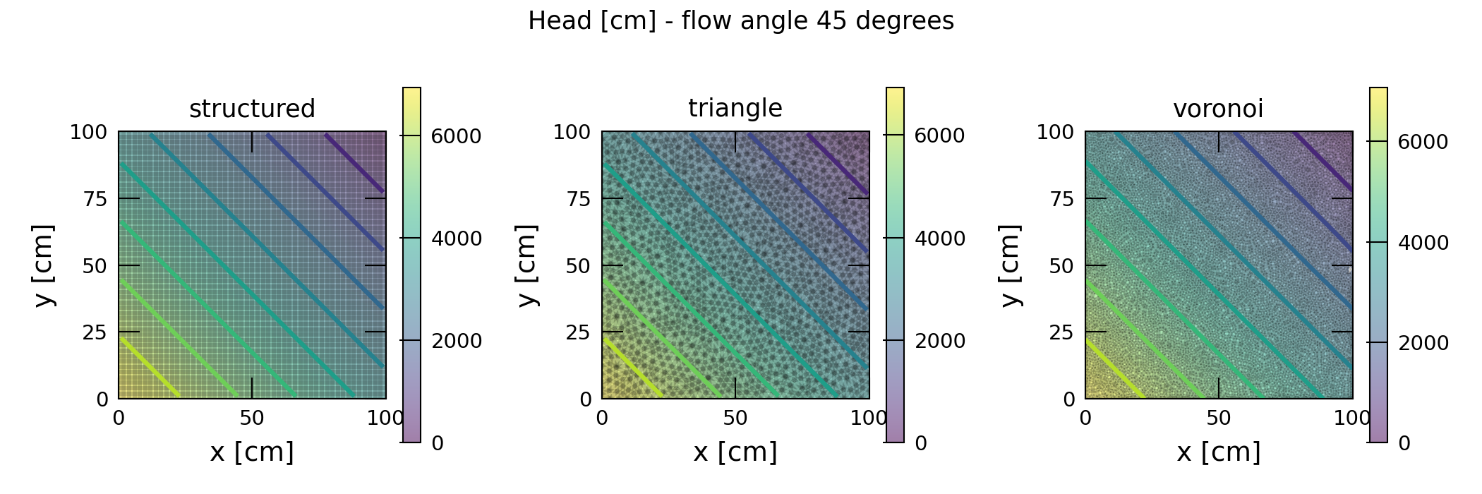
Figure 74.1 Computed head fields for the three grid types used in the advection scheme comparison. Left: Structured rectangular grid. Center: Triangular grid. Right: Voronoi polygon grid. All grids produce the expected uniform head gradient at a 45° angle.

74.2.2. Concentration Field Results

Figures Figure 74.2, Figure 74.3, and Figure 74.4 show the final concentration distributions at the end of the simulation, which are near the steady-state solution, for the three inflow concentration profiles across all scheme and grid combinations. These 2D concentration maps reveal the characteristic behavior of each numerical scheme, though the specific wave profiles are more clearly visualized in the cross-section analysis presented later. A mask has been applied to filter out all values below 0 and above 1. This has been done to make it easier to compare the results between different schemes.

74.2.2.1. Sin² wave results

(Figure 74.2) reveal important differences in scheme performance for this smooth inflow concentration profile. While all schemes perform well on the structured grid, the upstream scheme is noticeably more diffusive. The central difference scheme becomes unstable on the triangular and Voronoi grids. On the structured grid, the central difference scheme is the least diffusive but exhibits undershoots resulting in negative concentrations due to the relatively high Courant number (0.7); lowering the Courant number eliminates this behavior. The UTVD scheme demonstrates robust performance across all grid types, maintaining both accuracy and stability.

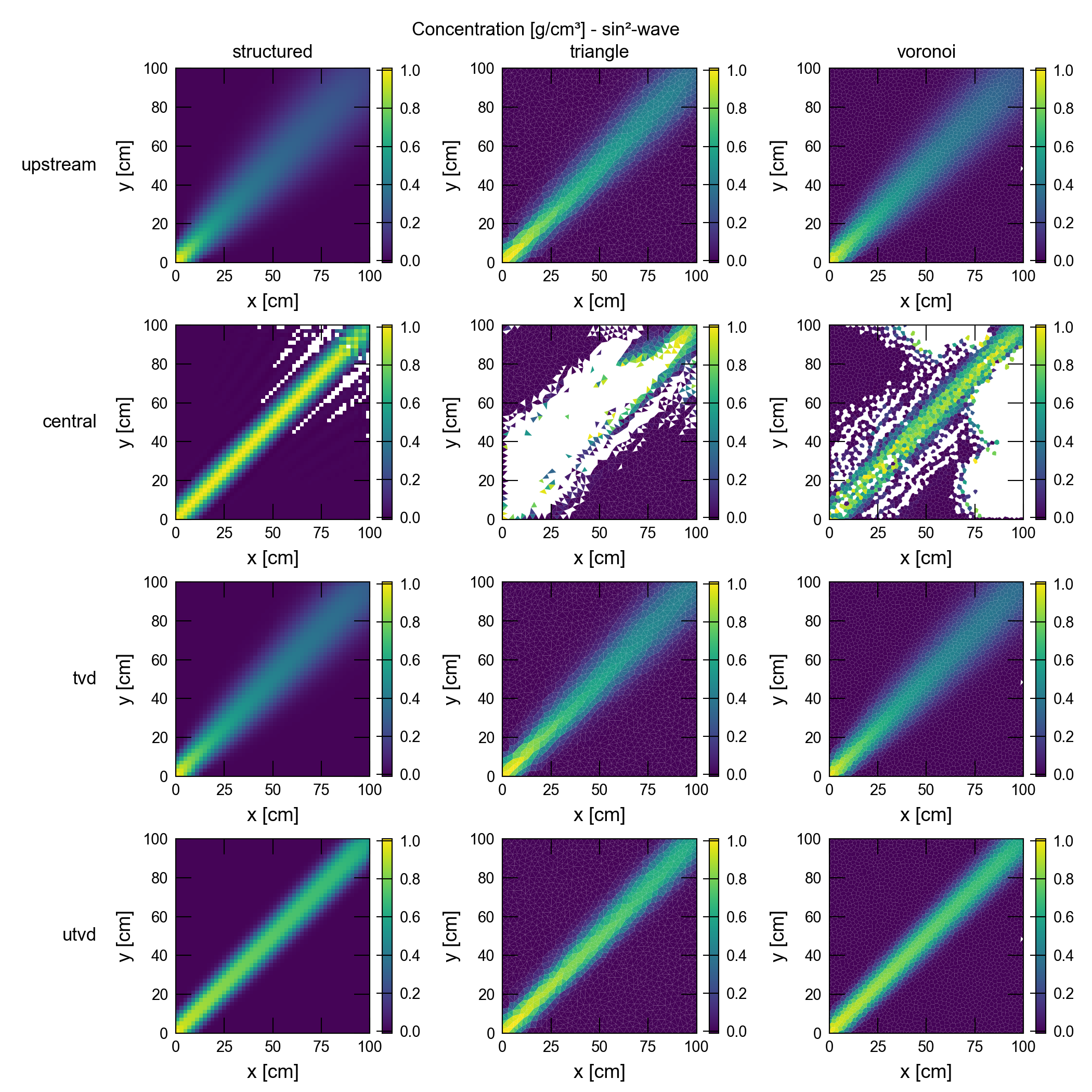
Figure 74.2 Final concentration distributions for the sin² wave inflow concentration profile. Rows represent the four advection schemes (upstream, central difference, TVD, UTVD) and columns represent the three grid types (structured, triangular, Voronoi).

74.2.2.2. Step wave results

(Figure 74.3) show similar trends to the sin² wave results. On the structured grid, the central difference scheme outperforms UTVD in preserving the overall shape of the wave. However, while it only exhibited undershoot for the smooth sin² wave, the sharp discontinuity of the step wave causes both undershoot and overshoot. For the step wave, the central difference scheme becomes unstable on the triangular and Voronoi grids. The TVD scheme outperforms upstream on the structured grid but performs similarly on the triangular and Voronoi grids. The UTVD scheme emerges as the least dissipative scheme that maintains stability across all grid types.

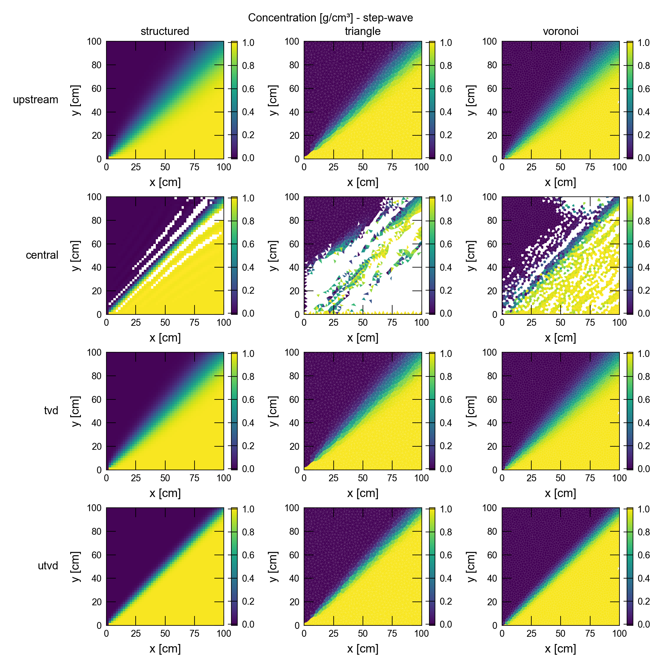
Figure 74.3 Final concentration distributions for the step wave inflow concentration profile. The central difference scheme begins to show oscillatory behavior near the sharp transition, while the TVD and UTVD schemes maintain stable solutions without spurious oscillations.

74.2.2.3. Square wave results

(Figure 74.4) exhibit similar behavior to the step wave results. The TVD scheme outperforms upstream on the structured grid but performs similarly on the triangular and Voronoi grids. The central difference scheme shows oscillations on the structured grid and blows up on the other grids. The UTVD scheme works well on all grids and is the only stable scheme that actually comes close to the maximum value of the analytical solution, demonstrating its capability for handling sharp discontinuities across all grid types.

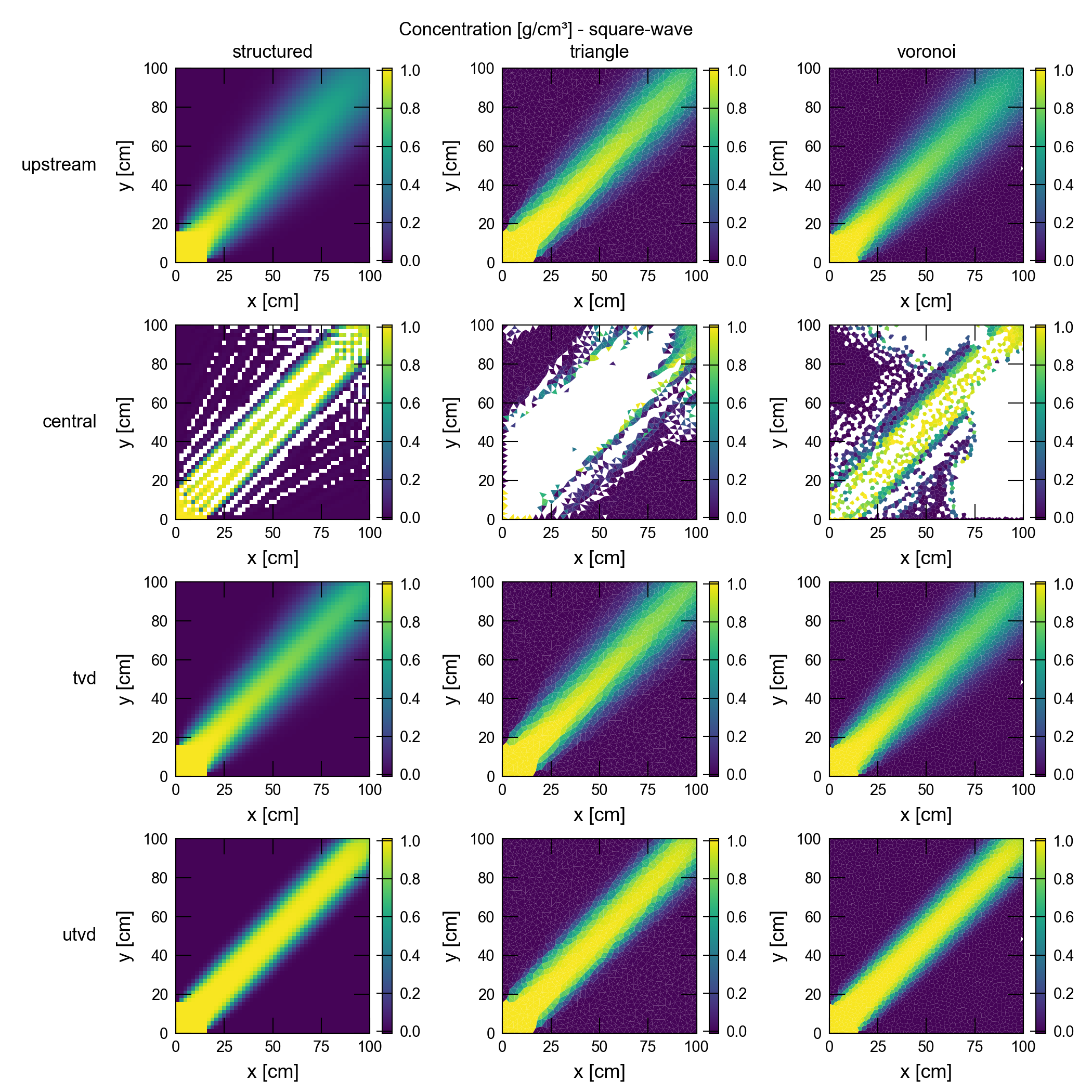
Figure 74.4 Final concentration distributions for the square wave inflow concentration profile. This test with sharp discontinuities demonstrates the oscillatory behavior of the central difference scheme and the ability of the TVD/UTVD schemes to maintain stable solutions without spurious oscillations.

74.2.3. Cross-Section Analysis

Figure 74.5 presents concentration profiles along the centerline (y = 50 cm) for all inflow concentration profiles and grid types, comparing numerical solutions against the analytical solution. These 1D cross-sections provide quantitative assessment of scheme accuracy and enable detailed comparison of numerical behavior:

Accuracy assessment: The cross-sections reveal that the UTVD scheme follows the analytical solution best for discontinuous functions, while maintaining computational stability. The TVD scheme only slightly outperforms the upstream scheme in terms of accuracy. The central difference scheme works well for the smooth function on a structured grid but its Courant condition is restricting, limiting its practical applicability.

Oscillation identification: Clear oscillations in the central difference scheme are visible as concentration values exceeding the physical bounds [0,1] or exhibiting spurious undershoot/overshoot behavior.

Grid sensitivity: The comparison across grid types demonstrates that UTVD maintains consistent performance regardless of grid geometry, while TVD may show some degradation on unstructured grids.

Diffusion quantification: The upstream scheme shows characteristic smearing of sharp features, providing a baseline for assessing the improvement offered by higher-order schemes.

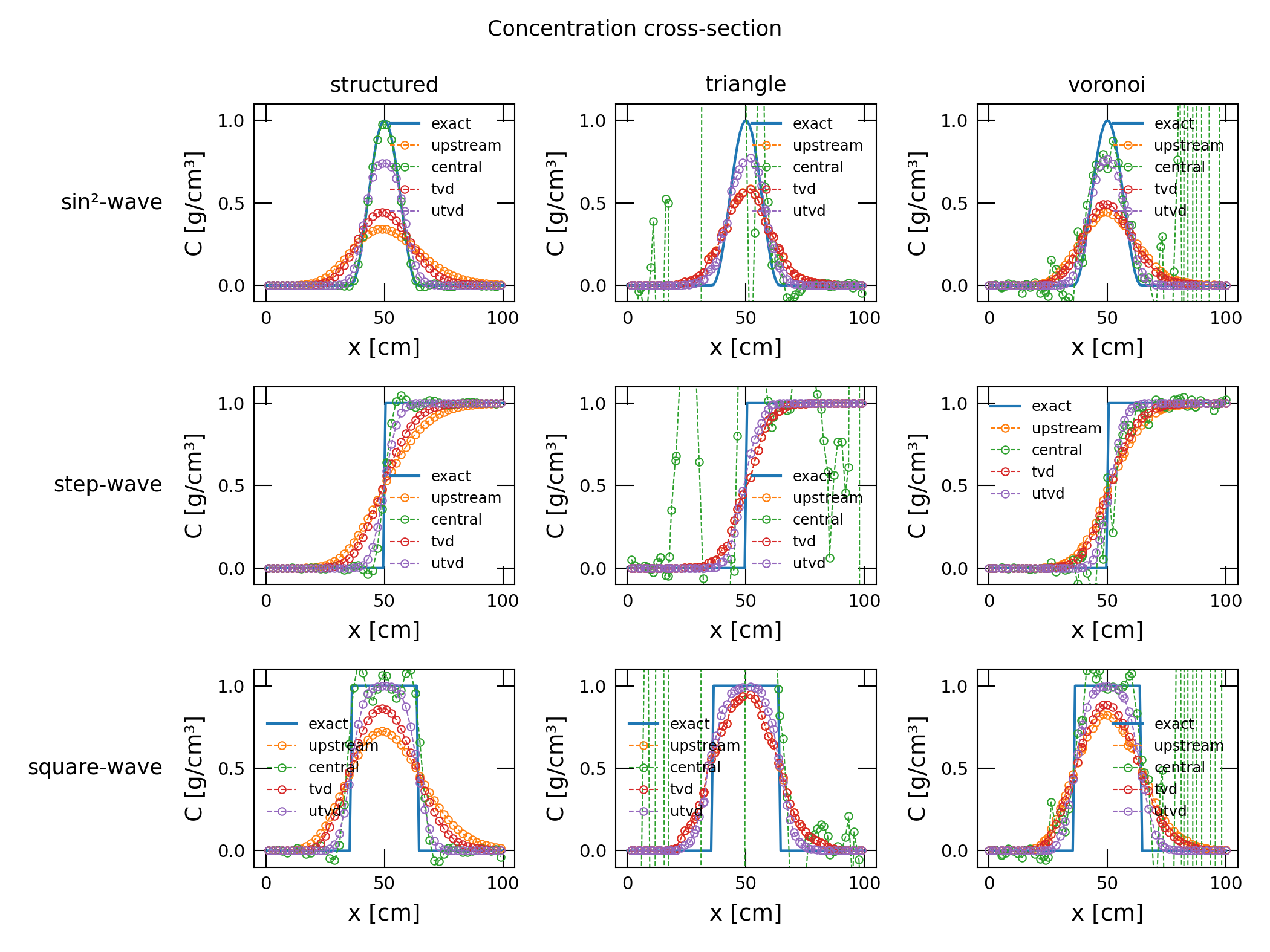
Figure 74.5 Concentration cross-sections at y = 50 cm comparing numerical solutions (dashed lines with markers) against analytical solutions (solid lines) for all inflow concentration profiles and grid types. Rows: Inflow concentration profiles (sin² wave, step wave, square wave). Columns: Grid types (structured, triangular, Voronoi). The restricted y-axis range [-0.1, 1.1] helps visualize oscillations and overshoots.

74.2.4. Key Findings

The results from these simulations provide several key findings that can be used as guidance for advection scheme selection in groundwater transport modeling. While this comparison is based on solid testing, it is also limited in scope and the findings should be interpreted accordingly:

1. Grid-dependent performance: The central difference scheme performed reasonably on the structured grid but became unstable on the triangular and Voronoi grids, particularly for the discontinuous input concentration profiles. This demonstrates the critical importance of considering grid type when selecting numerical schemes.

2. Courant number sensitivity: The central difference scheme’s stability was highly sensitive to the Courant number. At Courant = 0.7, it exhibited undershoots leading to negative concentrations on smooth functions and oscillartory instability for the discontinuous inflow concentration profiles. Reducing the Courant number mitigated these issues for the smooth inflow concentration profile but at the cost of computational efficiency.

3. UTVD scheme as overall best choice: The UTVD scheme consistently outperformed all others across grid types and inflow concentration profiles. It was the least dissipative scheme that maintained stability, and is the only stable scheme that approached the maximum values of analytical solutions for sharp discontinuities.

4. TVD limitations on unstructured grids: While TVD performed well on the structured grid and outperformed the upstream scheme for the discontinuous input concentration profiles, its advantage diminished on the unstructured grids, where it performed similarly to the upstream scheme.

5. Upstream scheme reliability: The upstream scheme provided a stable baseline across all grid types and inflow concentration profiles, though with significant diffusion. It can serve as a reliable fallback option when stability is paramount.

6. Practical recommendations: For unstructured grid applications involving transport with potential sharp fronts, the tests conducted here suggest that UTVD is the best choice. For structured grids, TVD offers a good balance of accuracy and stability. The central difference scheme should be used with caution and requires careful Courant number selection, particularly on unstructured grids. If computational speed is prioritized and users can accept more diffusive solutions, the upstream scheme provides a fast and stable option. Similarly, if users can tolerate potential instabilities in exchange for speed and higher accuracy on structured grids, the central difference scheme may be considered with appropriate Courant number restrictions.

74.3. Jupyter Notebook

The Jupyter notebook used to create the MODFLOW 6 input files for this example and post-process the results is:

• ex-gwt-adv-schemes