68. Thermal Loading of Borehole Heat Exchangers

Borehole Heat Exchangers (BHE’s) are increasingly used to provide a sustainable source of cooling and heating for buildings. The thermal energy demands may vary seasonally, with heat extraction occurring during the winter season and heat injection during the warmer summer months. As a result, the subsurface temperature near the BHE’s will show seasonal variability. This is illustrated here using the Groundwater Energy Transport (GWE) model. The results are compared with an analytical solution to verify the accuracy of the MODFLOW 6 simulation.

68.1. Example description

Five BHE’s are arbitrarily placed in a confined aquifer with uniform background flow in the x-direction. The BHE’s are fully screened across the aquifer thickness and heat injection/extraction is evenly distributed along the borehole length. The resulting temperature field therefore does not vary along the z-axis, effectively rendering the problem two-dimensional. Heat extraction and injection follow a seasonal energy demand typical for residential BHE systems in temperate climates (Figure 68.1). During winter, heat is extracted from the aquifer whereas heat is injected (or cold is extracted) during summer. Note that on a yearly basis, more heat is extracted than injected.

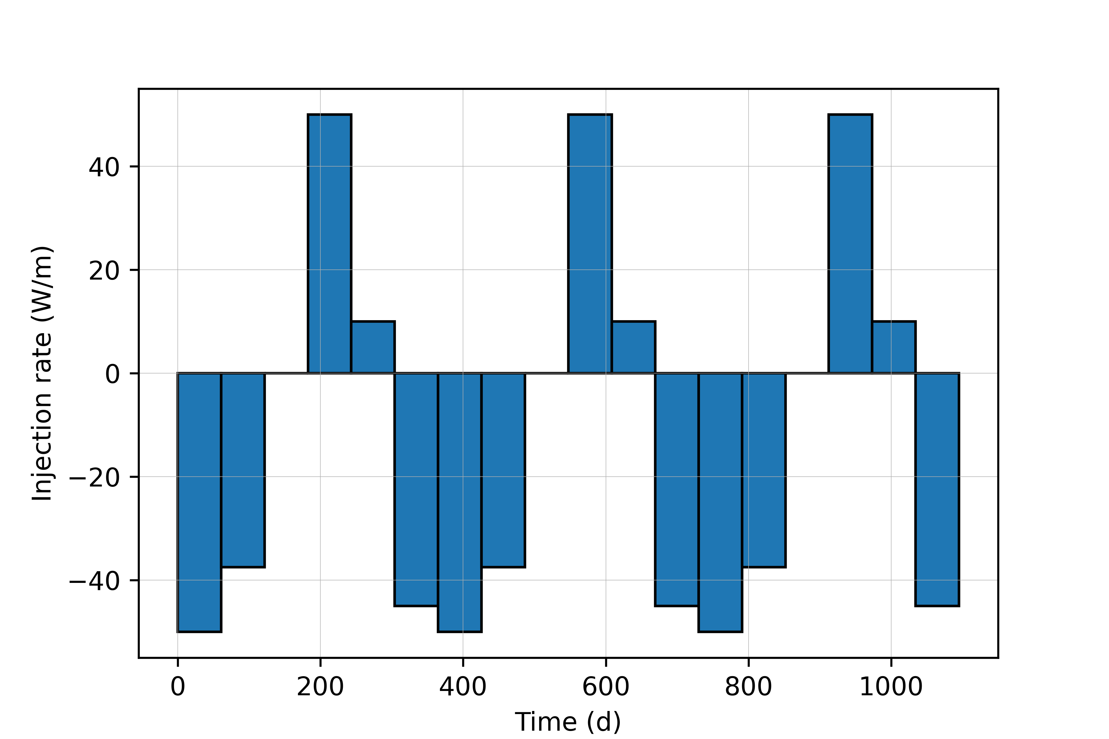
Figure 68.1 Heat injection rate per unit aquifer thickness for each BHE.

The MODFLOW 6 model consists of a single, confined layer of unit thickness to simulate the 2D system. The domain extent is 80 \(m\) \(\times\) 80 \(m\) and is discretized using rectangular cells of 1 \(m\) \(\times\) 1 \(m\). Flow is steady-state and uniform in the x-direction as implemented by constant-heads at the left and right boundaries. The BHE’s are placed in the center of the model using the Energy Source Loading (ESL) package with energy source loading rates varying every two months. This annual energy loading cycle is repeated for three years (Figure 68.1). Each loading phase is simulated using 10 time steps. The initial background temperature equals 0 \(^{\circ} C\), so the simulated temperature field represents the relative change in temperature compared to an arbitrary starting temperature. Thus, negative simulated temperatures do not represent a frozen condition, but rather a relative decrease in temperature. Model parameters are summarized in Table 68.1.

Table 68.1 Model parameters for example ex-gwe-bhe.

Parameter	Value
Length of system in X direction (\(m\))	80.0
Length of system in Y direction (\(m\))	80.0
Width along columns (\(m\))	1.0
Width along rows (\(m\))	1.0
Total number of layers (\(-\))	1
Aquifer top elevation (\(m\))	1.0
Aquifer bottom elevation (\(m\))	0.0
Aquifer hydraulic conductivity (\(m/d\))	10.0
Aquifer porosity (\(-\))	0.2
Advection solution scheme (\(-\))	TVD
Thermal conductivity of water (\(\frac{W}{m \cdot ^{\circ}C}\))	0.59
Thermal conductivity of aquifer material (\(\frac{W}{m \cdot ^{\circ}C}\))	2.5
Density of water (\(\frac{kg}{m^3}\))	1000.0
Heat capacity of water (\(\frac{J}{kg \cdot ^{\circ}C}\))	4184.0
Density of dry solid aquifer material (\(\frac{kg}{m^3}\))	2650.0
Heat capacity of dry solid aquifer material (\(\frac{J}{kg \cdot ^{\circ}C}\))	900.0
Longitudinal dispersivity (\(m\))	0.0
Horizontal transverse dispersivity (\(m\))	0.0
Initial temperature of the domain (\(^{\circ}C\))	0.0
Groundwater flow velocity (\(m/d\))	0.1

68.2. Analytical solution

An analytical solution for the described 2D problem can be derived based on the POINT2 algorithm provided by (Wexler, 1992) (equation 76) describing 2D solute transport for a continuous point source in an aquifer with uniform background flow:

(68.1)\[C(x,y,t) = \frac{C_0Q'}{4n\pi\sqrt{D_xD_y}}exp(\frac{v(x-x_c)}{2D_x})\int_0^t\frac{1}{\tau} exp(-\frac{v^2}{4D_x}\tau - \frac{(x-x_c)^2}{4D_x\tau}-\frac{(y-y_c)^2}{4D_y\tau})d\tau\]

By dividing \(v\), \(D_x\), \(D_y\) and \(Q'\) by the retardation coefficient \(R\), linear equilibrium sorption can be included.

Using the analogy between the solute transport equation and the heat transport equation (see e.g. (Zheng, 2010)), equation 68.1 can be used to simulate 2D heat transport from a continuous point source in an aquifer with uniform background flow by transforming the governing heat transport parameters into the solute transport parameters \(R\), \(D_m\) and \(C_0\):

(68.2)\[k_0 = n k_w + (1 - n) k_s\]

(68.3)\[D_m = \frac{k_0}{n \rho_w C_w}\]

(68.4)\[\rho_b = (1 - n) \rho_s\]

(68.5)\[K_d = \frac{C_s}{C_w \rho_w}\]

(68.6)\[R = 1 + \frac{K_d \rho_b}{n}\]

(68.7)\[Q' = 1\]

(68.8)\[C_0 = \frac{F_0}{\rho_w C_w}\]

where the heat injection rate \(F_0\) per unit aquifer thickness \([ET^{-1}L^{-1}]\) is converted to the injection concentration \(C_0\) and the injection rate per unit aquifer thickness \(Q'\) is set to unity. Since equation 68.1 is linear, the superposition principle can be applied to allow for multiple BHE’s in space as well as time-varying energy loading.

68.3. Example Results

Simulated temperature change contours after 1.5 years show that the groundwater temperature has decreased around the BHE field (Figure 68.2). This decrease has stretched in the direction of flow as the cooler groundwater is transported downgradient. A good agreement is found between the analytical solution and the MODFLOW 6 solution. A time series of the simulated temperature change at a location downgradient of the BHE field shows the seasonal variation in groundwater temperature (Figure 68.3). Since the annual heating demand is larger than the cooling demand, a thermal imbalance of the subsurface occurs during the early stages of operation. This causes the groundwater system to initially cool down before reaching a thermal dynamic equilibrium. As a result, the effectiveness of the residential heating is reduced in the long term as a larger temperature difference now needs to be met to sufficiently heat the building during winter, which needs to be taken into account when dimensioning the system. The MODFLOW 6 results again show a good agreement with the analytical solution.

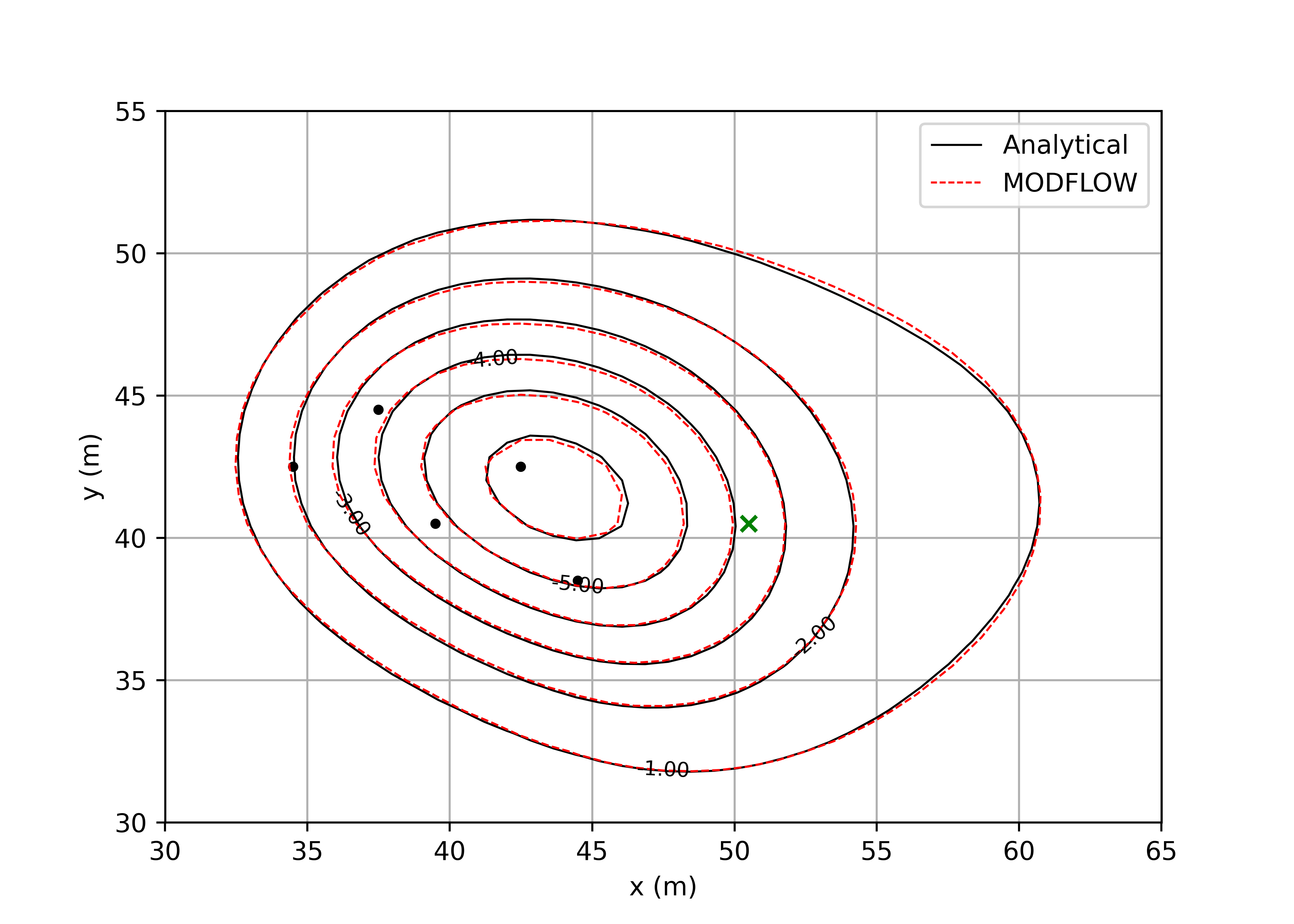
Figure 68.2 Contours of the simulated temperature change after 1.5 years using the MODFLOW 6 GWE model (dashed red line) and the analytical solution (solid black line). The green cross marks the location of the observation well in Figure 68.3. The black dots show the locations of the BHE’s.

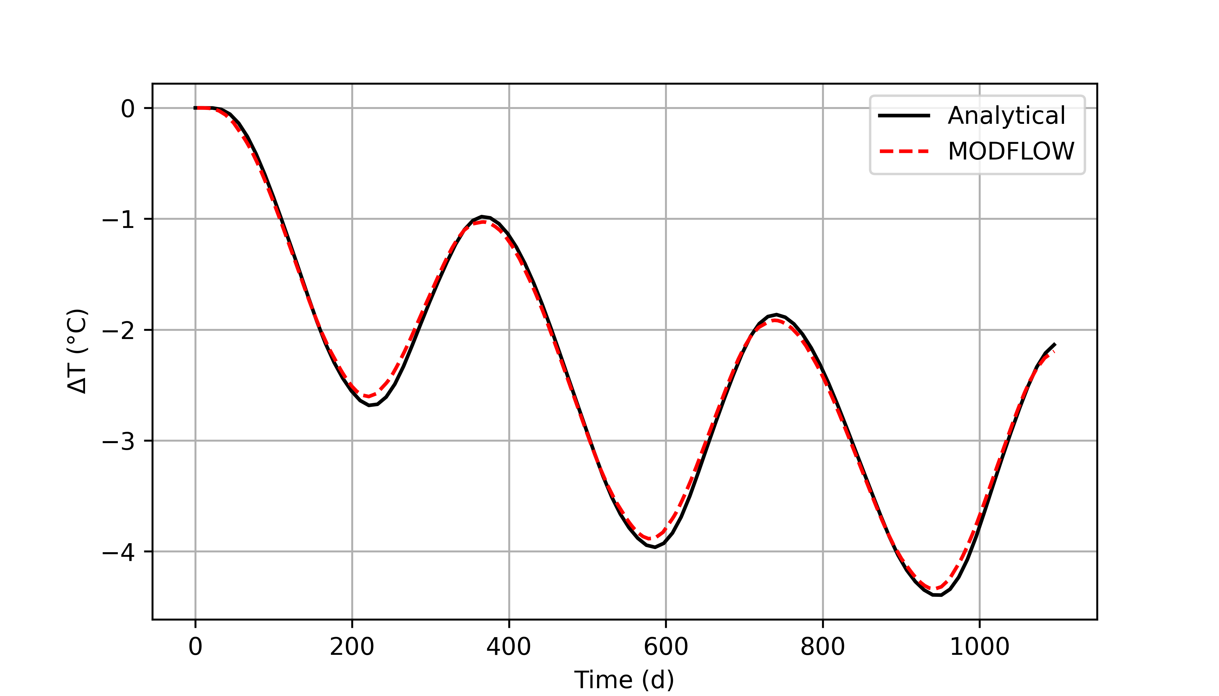
Figure 68.3 Time series of the simulated temperature change at the location shown in Figure 68.2 using the MODFLOW 6 GWE model (dashed red line) and the analytical solution (solid black line).

68.4. References Cited

Wexler, E. J. (1992). Analytical solutions for one-, two-, and three-dimensional solute transport in ground-water systems with uniform flow.

Zheng, C. (2010). MT3DMS v5.3—a modular three-dimensional multi-species transport model for simulation of advection, dispersion and chemical reactions of contaminants in groundwater systems; supplemental user’s guide.

68.5. Jupyter Notebook

The Jupyter notebook used to create the MODFLOW 6 input files for this example and post-process the results is:

• ex-gwe-bhe