Advection schemes in MODFLOW 6
This example demonstrates the performance of different numerical advection schemes when solving the groundwater transport equation under pure advection conditions. We solve the pure advection equation:
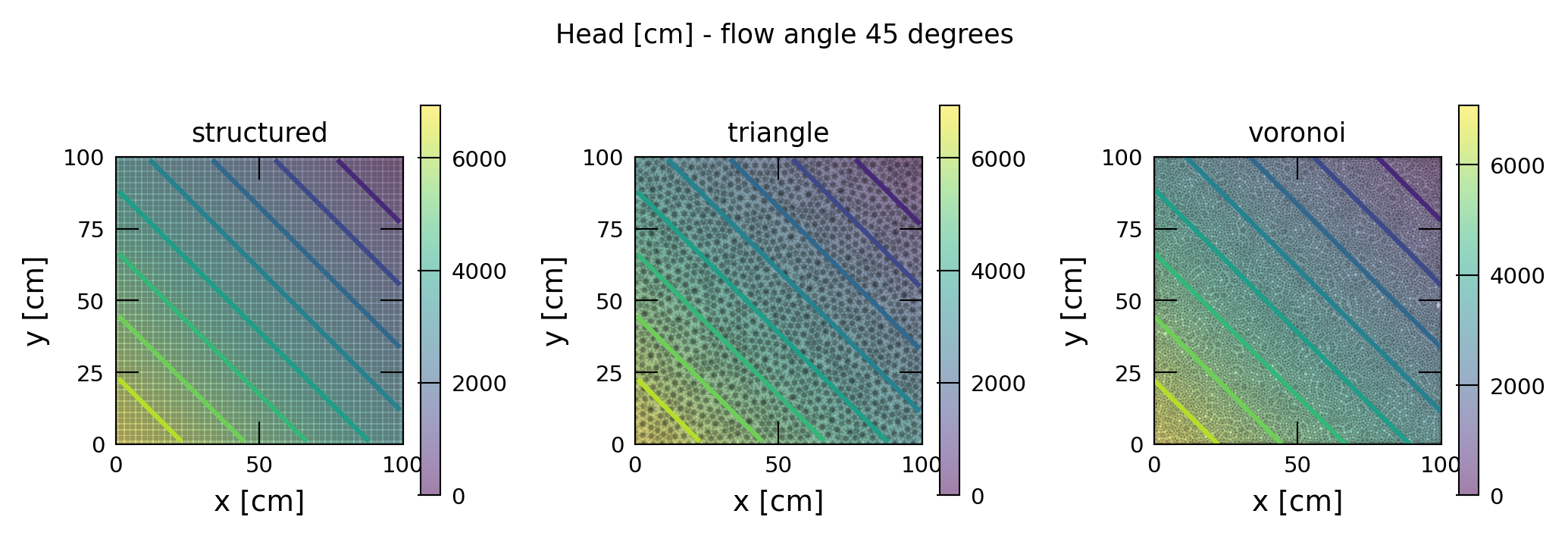
where C is concentration [g/cm³] and q is the specific discharge field = (qx, qy) = (0.354, 0.354) cm/s at 45°. The problem is configured with no dispersion or diffusion terms, making it a perfect test case for numerical scheme performance since an analytical solution exists.
Problem Setup:
Domain: 100cm x 100cm square with uniform flow at a 45° angle
Boundary conditions: Prescribed concentrations on inflow boundaries
Time: 300 seconds with adaptive time stepping (initial dt = 5s)
Physics: Pure advection without mixing processes (analytical solution available)
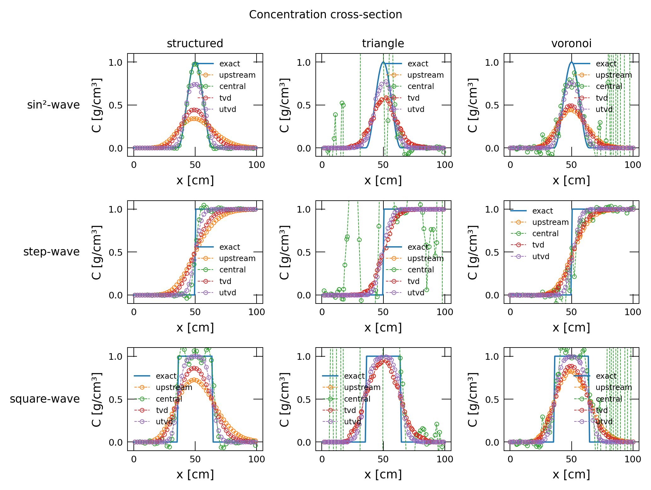
Four Advection Schemes Tested:
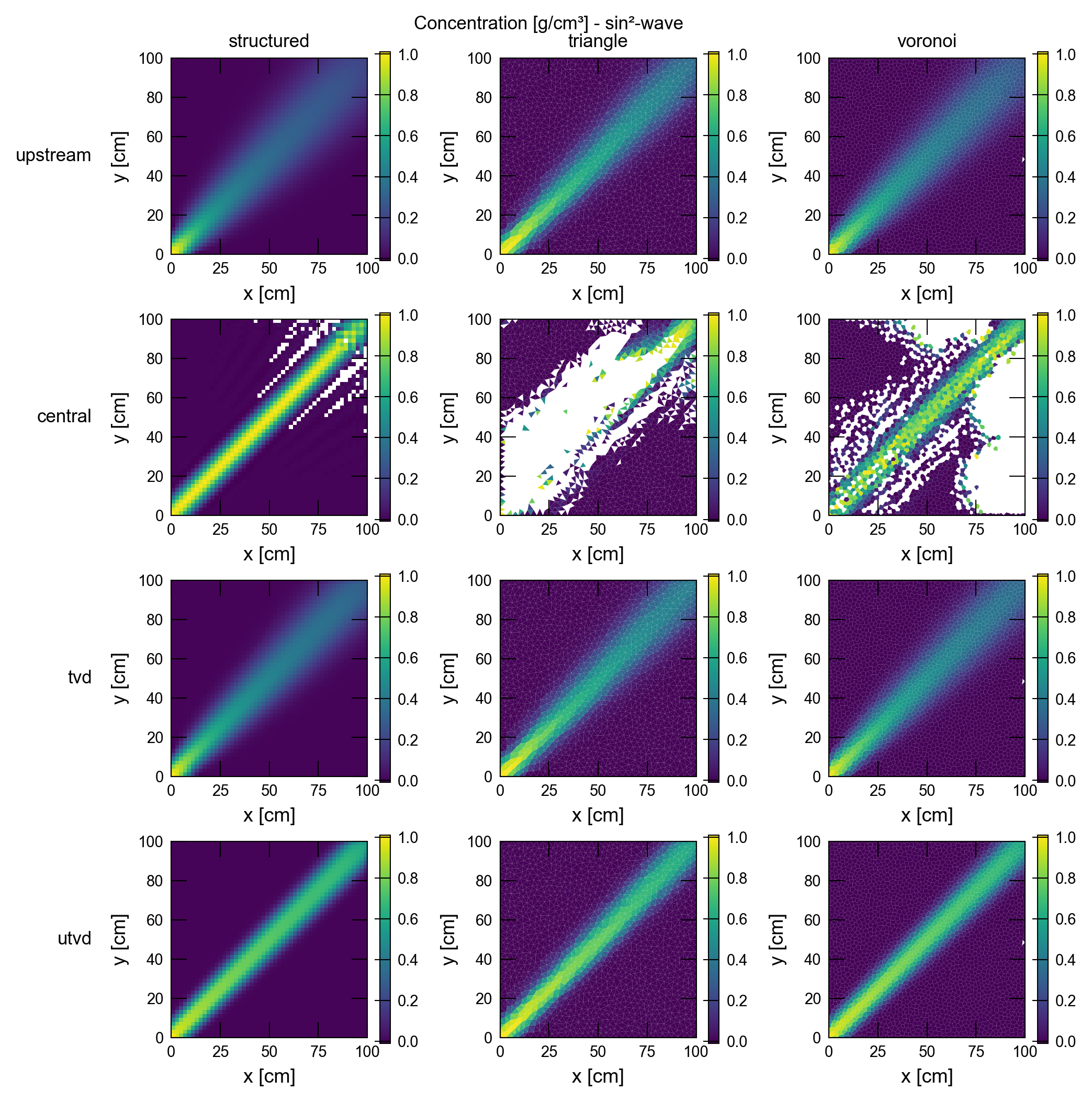
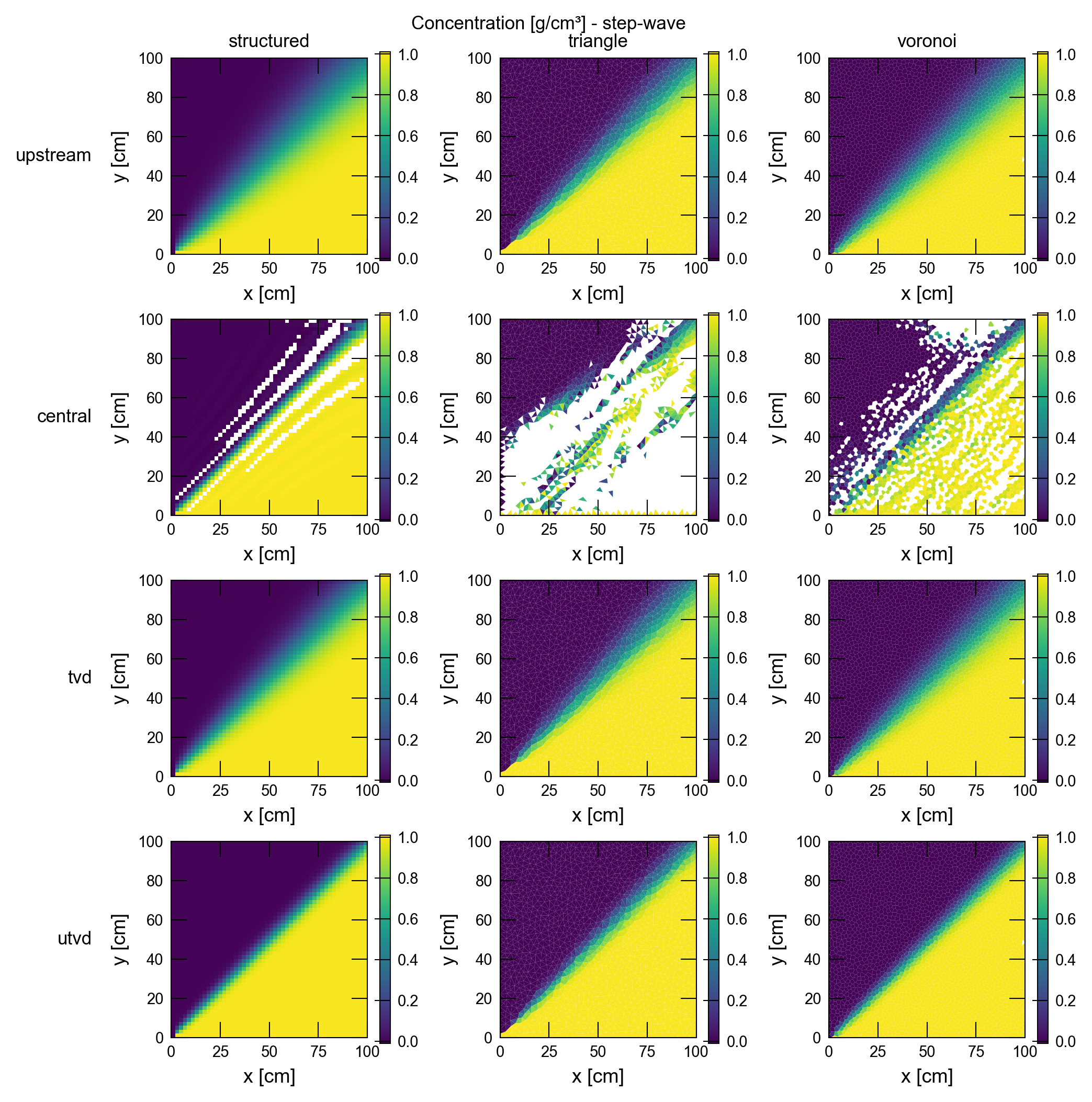
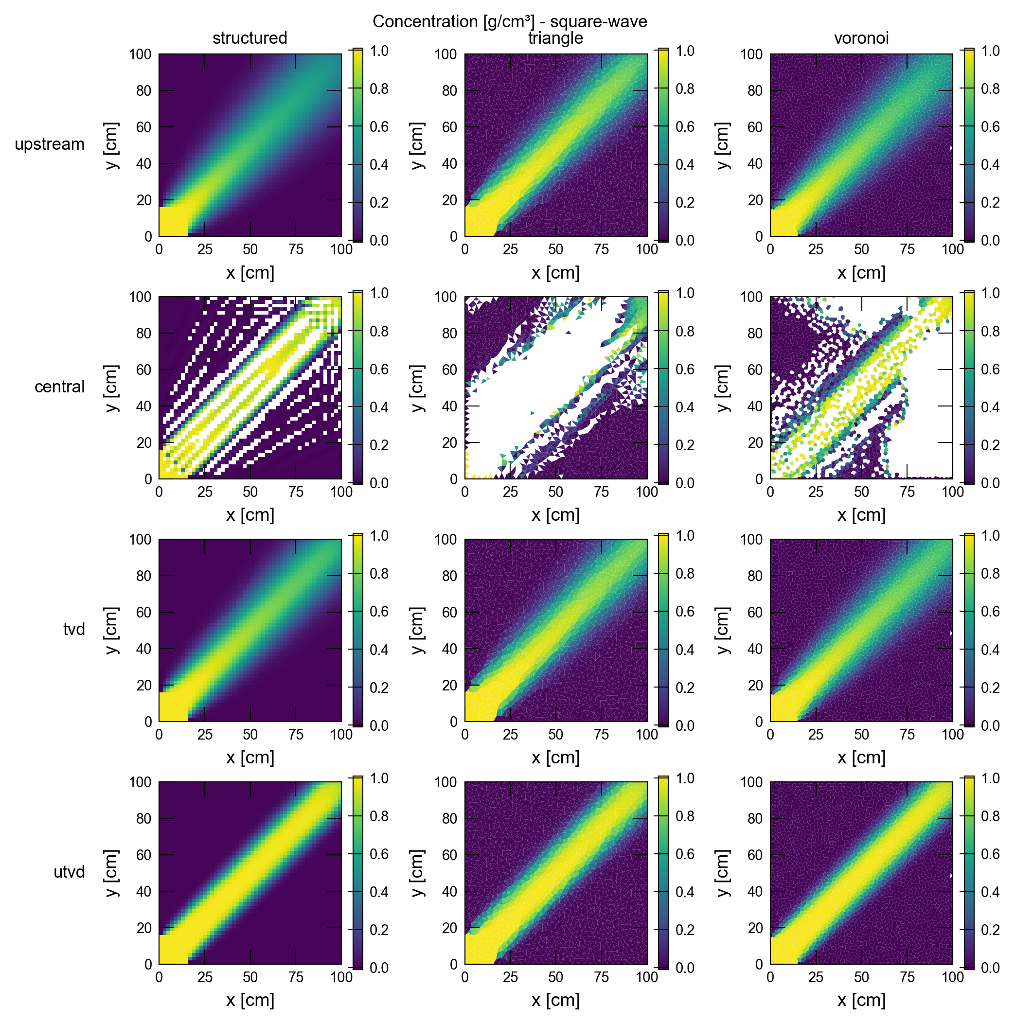
Upstream: 1st-order accurate, stable but diffusive
Central Difference (CD): 2nd-order accurate but can oscillate on discontinuities
TVD (Total Variation Diminishing): Handles sharp fronts well, works reliably only on structured grids
UTVD (Unstructured TVD): TVD extended with unstructured grid support, maintains TVD-quality performance on all grid types
Three Test Functions (probing different numerical challenges):
sin² wave: Smooth function testing 2nd-order accuracy
Square wave: Sharp discontinuity testing stability
Step wave: Sharp transition testing boundedness
Three Grid Types:
Structured: Regular rectangular cells
Triangle: Triangular mesh elements
Voronoi: Voronoi polygon cells
Expected Results:
CD scheme should oscillate/fail on discontinuous functions
TVD should work well on structured grids but may have issues on unstructured grids
UTVD should handle discontinuities without oscillation across all grid types
Different grid geometries may show different accuracy characteristics for the same numerical scheme
Initial setup
Import dependencies, define the example name and workspace, and read settings from environment variables.
[1]:
import collections.abc
import itertools
import math
from pathlib import Path

import flopy
import matplotlib.pyplot as plt
import numpy as np
import pandas as pd
from flopy.discretization.vertexgrid import VertexGrid
from flopy.plot.styles import styles
from flopy.utils import GridIntersect
from flopy.utils.triangle import Triangle
from flopy.utils.voronoi import VoronoiGrid
from modflow_devtools.misc import get_env, timed
from scipy.interpolate import LinearNDInterpolator
from shapely.geometry import LineString

try:
    import git
except ImportError:
    git = None

# Example name and workspace paths. If this example is running
# in the git repository, use the folder structure described in
# the README. Otherwise just use the current working directory.
sim_name = "ex-gwt-adv-schemes"
try:
    if git is not None:
        root = Path(git.Repo(".", search_parent_directories=True).working_dir)
    else:
        root = None
except Exception:
    root = None
workspace = root / "examples" if root else Path.cwd()
figs_path = root / "figures" if root else Path.cwd()

# Settings from environment variables
write = get_env("WRITE", True)
run = get_env("RUN", True)
plot = get_env("PLOT", True)
plot_show = get_env("PLOT_SHOW", True)
plot_save = get_env("PLOT_SAVE", True)
Define parameters
Define model units, parameters and other settings.
[2]:
# Model units
length_units = "centimeters"  # Length units
time_units = "seconds"  # Time units

# Model parameters
nper = 1  # Number of periods
nlay = 1  # Number of layers for the structured grid
ncol = 50  # Number of columns for the structured grid
nrow = 50  # Number of rows for the structured grid
Length = 100.0  # Domain length (cm)
Width = 100.0  # Domain width (cm)

delr = 2  # Column width (cm) for the structured grid
delc = 2  # Row width (cm) for the structured grid
top = 1.0  # Top elevation of the model (cm)
botm = 0  # Bottom elevation of the model (cm)

specific_discharge = 0.5  # Specific discharge (cm/s)
hydraulic_conductivity = 0.01  # Hydraulic conductivity (cm/s)
angledeg = 45  # Flow direction (°)
profile_width = 20.0  # Width of the inflow concentration profiles (cm)

total_time = 300.0  # Total simulation time (s)
dt = 5  # Initial time step (s)
percel = 0.7  # Courant number (-)

# Solver parameters
nouter = 100  # Maximum outer iterations
ninner = 300  # Maximum inner iterations
hclose = 1e-6  # Head closure criterion
cclose = 1e-6  # Concentration closure criterion
rclose = 1e-6  # Residual closure criterion

# Grid and scheme definitions
grids = ["structured", "triangle", "voronoi"]  # 3 grid types (36 total simulations)
schemes = ["upstream", "central", "tvd", "utvd"]  # 4 advection schemes
wave_functions = ["sin²-wave", "step-wave", "square-wave"]  # 3 test functions

# Abbreviations for model names (to fit MF6's 16-character limit)
grid_abbrev = {"structured": "s", "triangle": "t", "voronoi": "v"}
wave_abbrev = {"sin2-wave": "sin2", "step-wave": "step", "square-wave": "sqr"}
scheme_abbrev = {"upstream": "up", "central": "cen", "tvd": "tvd", "utvd": "utvd"}

# Compute discharge components
angle = math.radians(angledeg)
qx = specific_discharge * math.cos(angle)  # x-component of specific discharge (cm/s)
qy = specific_discharge * math.cos(angle)  # y-component of specific discharge (cm/s)

AXES_FRACTION = "axes fraction"
OFFSET_POINTS = "offset points"
Exact solution of the concentration field for pure advection.
The analytical solution works by:
Rotating coordinates to align with flow direction
Applying the 1D inlet signal in the rotated coordinate system
This works because advection simply translates the inlet pattern
For uniform flow at angle θ, any point (x,y) maps to:
Rotated coordinate: y’ = sin(-θ)·x + cos(-θ)·y
Concentration: C(x,y,t) = inlet_signal(y’ - v·t) Note: At t=300s, the pattern has fully advected through the domain
[3]:
def exact_solution_concentration(x, y, analytical):
    """Calculate exact concentration at any point in the domain.

    The analytical solution works by:
    1. Rotating coordinates to align with flow direction
    2. Applying the 1D inlet signal in the rotated coordinate system
    3. This works because advection simply translates the inlet pattern

    Args:
        x, y: Spatial coordinates (cm)
        analytical: Signal type ('sin²-wave', 'step-wave', 'square-wave')

    Returns:
        Concentration values [dimensionless, 0-1]
    """
    # Rotate to 1d solution space
    reverse_angle = -angle
    rotated_y = math.sin(reverse_angle) * x + math.cos(reverse_angle) * y

    # Compute concentration
    return inlet_signal(rotated_y, analytical)


def inlet_signal(y, signal_name):
    """Generate inlet signal based on the signal type.

    Args:
        y: y-coordinate values
        signal_name: Type of signal ('step-wave', 'square-wave', 'sin²-wave')

    Returns:
        Concentration values based on the signal type
    """
    clipped_y = np.clip(y, -profile_width / 2, profile_width / 2)
    match signal_name:
        case "step-wave":
            return np.where(y < 0, np.ones(y.shape), np.zeros(y.shape))
        case "square-wave":
            return np.where(
                np.abs(y) < profile_width / 2, np.ones(y.shape), np.zeros(y.shape)
            )
        case "sin²-wave":
            return np.power(np.cos(math.pi * clipped_y / profile_width), 2)
        case _:
            raise ValueError("Unknown signal name")
[4]:
def grid_triangulator(itri, delr, delc):
    nrow, ncol = itri.shape
    if np.isscalar(delr):
        delr = delr * np.ones(ncol)
    if np.isscalar(delc):
        delc = delc * np.ones(nrow)
    regular_grid = flopy.discretization.StructuredGrid(delc, delr)
    vertdict = {}
    icell = 0
    for i in range(nrow):
        for j in range(ncol):
            vs = regular_grid.get_cell_vertices(i, j)
            if itri[i, j] == 0:
                vertdict[icell] = [vs[0], vs[1], vs[2], vs[3], vs[0]]
                icell += 1
            elif itri[i, j] == 1:
                vertdict[icell] = [vs[0], vs[1], vs[3], vs[0]]
                icell += 1
                vertdict[icell] = [vs[3], vs[1], vs[2], vs[3]]
                icell += 1
            elif itri[i, j] == 2:
                vertdict[icell] = [vs[0], vs[2], vs[3], vs[0]]
                icell += 1
                vertdict[icell] = [vs[0], vs[1], vs[2], vs[0]]
                icell += 1
            else:
                raise ValueError(f"Unknown itri value: {itri[i, j]}")
    verts, iverts = flopy.utils.cvfdutil.to_cvfd(vertdict)
    return verts, iverts


def cvfd_to_cell2d(verts, iverts):
    vertices = []
    for i in range(verts.shape[0]):
        x = verts[i, 0]
        y = verts[i, 1]
        vertices.append([i, x, y])
    cell2d = []
    for icell2d, vs in enumerate(iverts):
        points = [tuple(verts[ip]) for ip in vs]
        xc, yc = flopy.utils.cvfdutil.centroid_of_polygon(points)
        cell2d.append([icell2d, xc, yc, len(vs), *vs])
    return vertices, cell2d


def grid_intersector(vgrid):
    """Create a grid intersector for the given vertex grid."""
    return flopy.utils.GridIntersect(vgrid)


def get_boundary(gi, line):
    line = LineString(line)
    cells = gi.intersect(line)["cellids"]
    cells = np.array(list(cells))

    return cells


def create_bc(boundary_ids, value, auxvalue=None):
    if auxvalue is None:
        if isinstance(value, collections.abc.Sequence | np.ndarray):
            return [
                [(0, cell_id), value[idx]] for idx, cell_id in enumerate(boundary_ids)
            ]
        else:
            return [[(0, cell_id), value] for idx, cell_id in enumerate(boundary_ids)]
    else:
        if isinstance(auxvalue, collections.abc.Sequence | np.ndarray):
            return [
                [(0, cell_id), value, auxvalue[idx]]
                for idx, cell_id in enumerate(boundary_ids)
            ]
        else:
            return [
                [(0, cell_id), value, auxvalue]
                for idx, cell_id in enumerate(boundary_ids)
            ]


def merge_bc_sum(boundaries):
    df = pd.DataFrame(boundaries)
    summed = df.groupby([0], as_index=False)[1].sum()

    return summed.values.tolist()


def merge_bc_mean(boundaries):
    df = pd.DataFrame(boundaries)
    mean = df.groupby([0], as_index=False)[1].mean()

    return mean.values.tolist()


def create_grid(grid_type, ws=None):
    """Create grid based on the specified type.

    Args:
        grid_type: Type of grid ('structured', 'triangle', 'voronoi')

    Returns:
        Tuple of (ncpl, nvert, vertices, cell2d)
    """
    if grid_type == "structured":
        itri = np.zeros((nrow, ncol), dtype=int)
        verts, iverts = grid_triangulator(itri, delr, delc)
        vertices, cell2d = cvfd_to_cell2d(verts, iverts)

        ncpl = len(cell2d)
        nvert = len(verts)

        return ncpl, nvert, vertices, cell2d
    elif grid_type == "triangle":
        active_domain = [(0, 0), (Length, 0), (Length, Width), (0, Width)]
        tri = Triangle(
            angle=30, maximum_area=delc * delr * 1.5, model_ws=ws or workspace
        )
        tri.add_polygon(active_domain)
        tri.build()

        cell2d = tri.get_cell2d()
        vertices = tri.get_vertices()
        ncpl = tri.ncpl
        nvert = tri.nvert

        return ncpl, nvert, vertices, cell2d
    elif grid_type == "voronoi":
        active_domain = [(0, 0), (Length, 0), (Length, Width), (0, Width)]
        tri = Triangle(
            angle=30, maximum_area=delc * delr / 1.5 * 1.2, model_ws=ws or workspace
        )
        tri.add_polygon(active_domain)
        tri.build()

        vor = VoronoiGrid(tri)
        disv_gridprops = vor.get_gridprops_vertexgrid()

        cell2d = disv_gridprops["cell2d"]
        vertices = disv_gridprops["vertices"]
        ncpl = disv_gridprops["ncpl"]
        nvert = len(vertices)

        return ncpl, nvert, vertices, cell2d

    else:
        raise ValueError(f"grid of type '{grid_type}' is not supported.")


def axis_aligned_segment_length(polygon, axis="y", value=0):
    """Calculate the total length of segments aligned with the specified axis at the given value."""
    total_length = 0.0
    coords = list(polygon.exterior.coords)

    for i in range(len(coords) - 1):
        p1, p2 = coords[i], coords[i + 1]
        is_aligned = (axis == "y" and p1[1] == value and p2[1] == value) or (
            axis == "x" and p1[0] == value and p2[0] == value
        )
        if is_aligned:
            segment = LineString([p1, p2])
            total_length += segment.length

    return total_length
Define functions to build models, write input files, and run the simulation.
[5]:
def build_mf6gwf(grid_type):
    gwfname = f"gwf_{grid_type}"
    sim_ws = workspace / sim_name / Path(gwfname)
    sim = flopy.mf6.MFSimulation(sim_name=sim_name, sim_ws=sim_ws, exe_name="mf6")

    tdis_ds = ((total_time, 1, 1.0),)
    flopy.mf6.ModflowTdis(sim, nper=nper, perioddata=tdis_ds, time_units=time_units)

    flopy.mf6.ModflowIms(
        sim,
        print_option="ALL",
        linear_acceleration="bicgstab",
        outer_maximum=nouter,
        outer_dvclose=hclose,
        inner_maximum=ninner,
        inner_dvclose=hclose,
        rcloserecord=rclose,
    )

    gwf = flopy.mf6.ModflowGwf(sim, modelname=gwfname, save_flows=True)

    flopy.mf6.ModflowGwfnpf(
        gwf,
        save_specific_discharge=True,
        save_saturation=True,
        export_array_ascii=True,
        xt3doptions=True,
        icelltype=0,
        k=hydraulic_conductivity,
    )

    flopy.mf6.ModflowGwfic(gwf, strt=0.0, export_array_ascii=True)

    ncpl, nvert, vertices, cell2d = create_grid(grid_type, ws=sim_ws)
    flopy.mf6.ModflowGwfdisv(
        gwf,
        nlay=nlay,
        ncpl=ncpl,
        nvert=nvert,
        top=top,
        botm=botm,
        vertices=vertices,
        cell2d=cell2d,
        filename=f"{gwfname}.disv",
    )

    head_filerecord = f"{gwfname}.hds"
    budget_filerecord_csv = f"{gwfname}.bud.csv"
    budget_filerecord = f"{gwfname}.bud"
    flopy.mf6.ModflowGwfoc(
        gwf,
        head_filerecord=head_filerecord,
        budgetcsv_filerecord=budget_filerecord_csv,
        budget_filerecord=budget_filerecord,
        saverecord=[("HEAD", "ALL"), ("BUDGET", "ALL")],
    )

    # Boundary lines
    bottom_edge = [(0, 0), (Length, 0)]
    right_edge = [(Length, 0), (Length, Width)]
    top_edge = [(Length, Width), (0, Width)]
    left_edge = [(0, Width), (0, 0)]

    # Identify boundary ids
    vgrid = VertexGrid(vertices=vertices, cell2d=cell2d, ncpl=ncpl, nlay=1)
    gi = grid_intersector(vgrid)

    bottom_boundary_ids = get_boundary(gi, bottom_edge)
    right_boundary_ids = get_boundary(gi, right_edge)
    top_boundary_ids = get_boundary(gi, top_edge)
    left_boundary_ids = get_boundary(gi, left_edge)

    # Set top right element to a chd 0. This makes the solution unique
    geometry = vgrid.geo_dataframe.geometry

    topright_id, _, _ = np.intersect1d(
        right_boundary_ids, top_boundary_ids, return_indices=True
    )

    if not topright_id.any():
        topright_id = [
            geometry.loc[top_boundary_ids].get_coordinates()["x"].idxmax().tolist()
        ]

    flopy.mf6.ModflowGwfchd(gwf, stress_period_data=create_bc(topright_id, 0))

    # Set boundary conditions
    cell_area = geometry.area.values
    inflow_area_left = (
        geometry.loc[left_boundary_ids]
        .apply(lambda poly: axis_aligned_segment_length(poly, axis="x", value=0))
        .values
    )
    inflow_area_bot = (
        geometry.loc[bottom_boundary_ids]
        .apply(lambda poly: axis_aligned_segment_length(poly, axis="y", value=0))
        .values
    )
    outflow_area_right = (
        geometry.loc[right_boundary_ids]
        .apply(lambda poly: axis_aligned_segment_length(poly, axis="x", value=Length))
        .values
    )
    outflow_area_top = (
        geometry.loc[top_boundary_ids]
        .apply(lambda poly: axis_aligned_segment_length(poly, axis="y", value=Width))
        .values
    )

    flopy.mf6.ModflowGwfrch(
        gwf,
        stress_period_data=merge_bc_sum(
            create_bc(
                left_boundary_ids, qx * inflow_area_left / cell_area[left_boundary_ids]
            )
            + create_bc(
                bottom_boundary_ids,
                qy * inflow_area_bot / cell_area[bottom_boundary_ids],
            )
            + create_bc(
                right_boundary_ids,
                -qx * outflow_area_right / cell_area[right_boundary_ids],
            )
            + create_bc(
                top_boundary_ids, -qy * outflow_area_top / cell_area[top_boundary_ids]
            )
        ),
    )

    return sim


def convert_superscript(text):
    map = {
        "¹": "1",
        "²": "2",
        "³": "3",
    }
    trans_table = str.maketrans(
        "".join(map.keys()),
        "".join(map.values()),
    )
    return text.translate(trans_table)


def build_mf6gwt(grid_type, scheme, wave_func):
    # Use abbreviated names for model name (16-char MF6 limit)
    wave_converted = convert_superscript(wave_func)
    gwtname = f"gwt_{grid_abbrev[grid_type]}_{wave_abbrev[wave_converted]}_{scheme_abbrev[scheme]}"
    # Use descriptive name for workspace
    pathname = f"gwt_{grid_type}_{wave_converted}_{scheme}"
    gwfname = f"gwf_{grid_type}"
    sim_ws = workspace / sim_name / Path(pathname)
    sim = flopy.mf6.MFSimulation(sim_name=sim_name, sim_ws=sim_ws, exe_name="mf6")

    nsteps = int(total_time / dt)
    tdis_ds = ((total_time, nsteps, 1.0),)

    tdis = flopy.mf6.ModflowTdis(
        sim, nper=nper, perioddata=tdis_ds, time_units=time_units
    )

    dtmin = 1e-5
    dtmax = 10
    dtadj = 2
    dtfailadj = dtadj
    ats_filerecord = gwtname + ".ats"
    atsperiod = [(0, dt, dtmin, dtmax, dtadj, dtfailadj)]
    tdis.ats.initialize(
        maxats=len(atsperiod),
        perioddata=atsperiod,
        filename=ats_filerecord,
    )

    flopy.mf6.ModflowIms(
        sim,
        linear_acceleration="bicgstab",
        print_option="SUMMARY",
        outer_maximum=nouter,
        outer_dvclose=cclose,
        inner_maximum=ninner,
        inner_dvclose=cclose,
        rcloserecord=rclose,
    )

    gwt = flopy.mf6.ModflowGwt(sim, modelname=gwtname, save_flows=True)

    flopy.mf6.ModflowGwtmst(gwt, porosity=1.0)

    flopy.mf6.ModflowGwtssm(gwt)

    flopy.mf6.ModflowGwtadv(gwt, scheme=scheme, ats_percel=percel)

    packagedata = [
        ("GWFHEAD", f"../{gwfname}/{gwfname}.hds", None),
        ("GWFBUDGET", f"../{gwfname}/{gwfname}.bud", None),
    ]
    flopy.mf6.ModflowGwtfmi(gwt, packagedata=packagedata, save_flows=True)

    flopy.mf6.ModflowGwtoc(
        gwt,
        budget_filerecord=f"{gwtname}.cbc",
        concentration_filerecord=f"{gwtname}.ucn",
        saverecord=[("CONCENTRATION", "LAST"), ("BUDGET", "LAST")],
        printrecord=[("CONCENTRATION", "LAST"), ("BUDGET", "LAST")],
    )

    ncpl, nvert, vertices, cell2d = create_grid(grid_type, ws=sim_ws)
    flopy.mf6.ModflowGwtdisv(
        gwt,
        nlay=nlay,
        ncpl=ncpl,
        nvert=nvert,
        top=top,
        botm=botm,
        vertices=vertices,
        cell2d=cell2d,
        filename=f"{gwtname}.disv",
    )

    # Boundary lines
    bottom_edge = [(0, 0), (Length, 0)]
    left_edge = [(0, Width), (0, 0)]

    # Identify boundary ids
    vgrid = VertexGrid(vertices=vertices, cell2d=cell2d, ncpl=ncpl, nlay=1)
    gi = grid_intersector(vgrid)

    bottom_boundary_ids = get_boundary(gi, bottom_edge)
    left_boundary_ids = get_boundary(gi, left_edge)

    # Compute exact solution for the inlet boundaries
    cell2d_df = pd.DataFrame(cell2d)
    xc, yc = cell2d_df.loc[bottom_boundary_ids, 1:2].T.to_numpy()
    conc_bottom = exact_solution_concentration(xc, yc, wave_func)
    xc, yc = cell2d_df.loc[left_boundary_ids, 1:2].T.to_numpy()
    conc_left = exact_solution_concentration(xc, yc, wave_func)

    # Set inlet concentrations
    flopy.mf6.ModflowGwtcnc(
        gwt,
        stress_period_data=merge_bc_mean(
            create_bc(bottom_boundary_ids, conc_bottom)
            + create_bc(left_boundary_ids, conc_left)
        ),
    )

    # Set initial condition equal to zero
    flopy.mf6.ModflowGwtic(gwt, strt=0)

    return sim
[6]:
def write_models(sim, silent=True):
    sim.write_simulation(silent=silent)


@timed
def run_models(sim, silent=True):
    success, buff = sim.run_simulation(silent=silent)
    assert success, buff
Define functions to plot model results.
[7]:
def plot_results(gwf_sims, gwt_sims):
    plot_flows(gwf_sims)
    plot_concentrations(gwt_sims)
    plot_concentration_cross_sections(gwt_sims)


def plot_flows(gwf_sims):
    with styles.USGSPlot():
        figure_size = (7, 7 / len(gwf_sims))
        fig, axs = plt.subplots(
            1, len(gwf_sims), dpi=300, figsize=figure_size, tight_layout=True
        )
        fig.suptitle("Head [cm] - flow angle 45 degrees")

        for idx, (grid, sim) in enumerate(gwf_sims.items()):
            plot_flow(sim, axs[idx])

        pad = 5  # in points
        for ax, col in zip(axs, gwf_sims.keys()):
            ax.annotate(
                col,
                xy=(0.5, 1),
                xytext=(0, pad),
                xycoords=AXES_FRACTION,
                textcoords=OFFSET_POINTS,
                size="large",
                ha="center",
                va="baseline",
            )

    if plot_show:
        plt.show()
    if plot_save:
        fname = f"{sim_name}-flow.png"
        fpth = figs_path / fname
        fig.savefig(fpth)


def plot_flow(sim, ax):
    gwf = sim.get_model()
    head = gwf.output.head().get_data()
    bud = gwf.output.budget()
    spdis = bud.get_data(text="DATA-SPDIS")[0]
    vmin = head.min()
    vmax = head.max()

    pmv = flopy.plot.PlotMapView(gwf, ax=ax)
    pmv.plot_grid(colors="k", alpha=0.1)
    pc = pmv.plot_array(head, vmin=vmin, vmax=vmax, alpha=0.5)
    pmv.contour_array(head, levels=np.linspace(vmin, vmax, 10))
    plt.colorbar(pc)

    ax.set_xlabel("x [cm]")
    ax.set_ylabel("y [cm]")
    ax.set_aspect("equal")


def plot_concentrations(gwt_sims):
    for wave_func in wave_functions:
        with styles.USGSPlot():
            fig, axs = plt.subplots(
                nrows=len(schemes),
                ncols=len(grids),
                dpi=300,
                figsize=(7, 7 * len(schemes) / (len(grids) + 1)),
                tight_layout=True,
            )
            fig.suptitle(f"Concentration [g/cm³] - {wave_func}")

            for idx_scheme, scheme in enumerate(schemes):
                for idx_grid, grid in enumerate(grids):
                    sim = gwt_sims[(grid, scheme, wave_func)]
                    plot_concentration(sim, axs[idx_scheme, idx_grid])

            pad = 5  # in points
            for ax, col in zip(axs[0], grids):
                ax.annotate(
                    col,
                    xy=(0.5, 1),
                    xytext=(0, pad),
                    xycoords=AXES_FRACTION,
                    textcoords=OFFSET_POINTS,
                    size="large",
                    ha="center",
                    va="baseline",
                )

            for ax, row in zip(axs[:, 0], schemes):
                ax.annotate(
                    row,
                    xy=(0, 0.5),
                    xytext=(-ax.yaxis.labelpad - pad, 0),
                    xycoords=ax.yaxis.label,
                    textcoords=OFFSET_POINTS,
                    size="large",
                    ha="right",
                    va="center",
                )

            fig.subplots_adjust(left=0.25, top=0.95)

            if plot_show:
                plt.show()
            if plot_save:
                fname = f"{sim_name}-{convert_superscript(wave_func)}-conc.png"
                fpth = figs_path / fname
                fig.savefig(fpth)


def plot_concentration(sim, ax):
    gwt = sim.get_model()
    ucnobj_mf6 = gwt.output.concentration()
    conc = ucnobj_mf6.get_data(totim=ucnobj_mf6.get_times()[-1]).flatten()

    tol = 1e-2
    vmin = -0.0 - tol
    vmax = 1.0 + tol

    masked_conc = np.ma.masked_outside(conc, vmin, vmax)
    pmv = flopy.plot.PlotMapView(gwt, ax=ax)
    pc = pmv.plot_array(masked_conc, vmin=vmin, vmax=vmax, alpha=1)
    plt.colorbar(pc)

    ax.set_xlabel("x [cm]")
    ax.set_ylabel("y [cm]")
    ax.set_aspect("equal")


def plot_concentration_cross_sections(gwt_sims):
    with styles.USGSPlot():
        fig, axs = plt.subplots(
            nrows=len(wave_functions),
            ncols=len(grids),
            dpi=300,
            figsize=(7, 7 * len(wave_functions) / (len(grids) + 1)),
            tight_layout=True,
        )
        fig.suptitle("Concentration cross-section")

        for wave_idx, wave_func in enumerate(wave_functions):
            for grid_idx, grid in enumerate(grids):
                ax = axs[wave_idx][grid_idx]
                plot_concentration_analytical(wave_func, ax)
                for scheme in schemes:
                    sim = gwt_sims[(grid, scheme, wave_func)]
                    plot_concentration_cross_section(sim, scheme, ax)

                ax.legend(fontsize="small")
                ax.set_xlabel("x [cm]")
                ax.set_ylabel("C [g/cm³]")
                ax.set_ylim(-0.1, 1.1)

        pad = 5  # in points
        for ax, col in zip(axs[0], grids):
            ax.annotate(
                col,
                xy=(0.5, 1),
                xytext=(0, pad),
                xycoords=AXES_FRACTION,
                textcoords=OFFSET_POINTS,
                size="large",
                ha="center",
                va="baseline",
            )

        for ax, row in zip(axs[:, 0], wave_functions):
            ax.annotate(
                row,
                xy=(0, 0.5),
                xytext=(-ax.yaxis.labelpad - pad, 0),
                xycoords=ax.yaxis.label,
                textcoords=OFFSET_POINTS,
                size="large",
                ha="right",
                va="center",
            )

        fig.subplots_adjust(left=0.25, top=0.95)

    if plot_show:
        plt.show()
    if plot_save:
        fname = f"{sim_name}-conc-cross-section.png"
        fpth = figs_path / fname
        fig.savefig(fpth)


def plot_concentration_analytical(analytical_func, ax):
    x = np.linspace(0, Length, 100)
    y = Width / 2

    conc = exact_solution_concentration(x, y, analytical_func)

    ax.plot(
        x, conc, linestyle="-", mfc="none", markersize="3", linewidth=1, label="exact"
    )


def plot_concentration_cross_section(sim, scheme, ax):
    gwt = sim.get_model()
    ucnobj_mf6 = gwt.output.concentration()
    conc = ucnobj_mf6.get_data(totim=ucnobj_mf6.get_times()[-1]).flatten()

    grid = gwt.modelgrid
    xc = grid.xcellcenters
    yc = grid.ycellcenters

    ix = GridIntersect(grid)
    x_line = LineString([(0, Width / 2), (Length, Width / 2)])
    xi = ix.intersect(x_line)
    x_along_line = sorted(xc[xi.cellids.tolist()])

    interp = LinearNDInterpolator(list(zip(xc, yc)), conc)
    conc_interp = interp([(i, Width / 2) for i in x_along_line])

    ax.plot(
        x_along_line,
        conc_interp,
        linestyle="--",
        marker="o",
        mfc="none",
        markersize="3",
        linewidth="0.5",
        markeredgewidth="0.5",
        label=scheme,
    )
Define and invoke a function to run the example scenario, then plot results.
[8]:
def scenario(silent=True):
    print("=" * 60)
    print("MODFLOW 6 Advection Schemes Comparison")
    print("=" * 60)
    print(
        f"Total simulations: {len(grids)} grids x {len(schemes)} schemes x {len(wave_functions)} functions = {len(grids) * len(schemes) * len(wave_functions)} transport models"
    )
    print(f"Plus {len(grids)} flow models")
    print()

    gwf_sims = {}

    # Build and run the gwt models on different grids
    for grid in grids:
        gwf_sims[grid] = build_mf6gwf(grid)

    # Build the gwt models
    gwt_sims = {}
    combinations = list(itertools.product(*[grids, schemes, wave_functions]))
    for combination in combinations:
        gwt_sims[combination] = build_mf6gwt(
            combination[0], combination[1], combination[2]
        )

    if write:
        print("\nWriting flow models:")
        for grid, sim in gwf_sims.items():
            print(f"- {grid} grid")
            write_models(sim, silent=silent)

        print("\nWriting transport models:")
        for key, sim in gwt_sims.items():
            grid, scheme, wave = key
            print(f"- {grid} grid \t {scheme} scheme \t {wave} function")
            write_models(sim, silent=silent)

    if run:
        print("\nRunning flow models:")
        for grid, sim in gwf_sims.items():
            print(f"- {grid} grid")
            run_models(sim, silent=silent)

        print("\nRunning transport models:")
        for key, sim in gwt_sims.items():
            grid, scheme, wave = key
            print(f"- {grid} grid \t {scheme} scheme \t {wave} function")
            run_models(sim, silent=silent)
    if plot:
        print("\n" + "=" * 40)
        print("PLOTTING RESULTS")
        print("=" * 40)
        print("Generating 3 figure sets:")
        print("1. Flow fields (3 subplots)")
        print(
            f"2. Concentration maps ({len(schemes)} rows x {len(grids)} cols per wave func = {len(schemes) * len(grids) * len(wave_functions)} total subplots)"
        )
        print(
            f"3. Cross-section comparisons ({len(wave_functions)} rows x {len(grids)} cols = {len(wave_functions) * len(grids)} subplots)"
        )
        plot_results(gwf_sims, gwt_sims)


scenario()
============================================================
MODFLOW 6 Advection Schemes Comparison
============================================================
Total simulations: 3 grids x 4 schemes x 3 functions = 36 transport models
Plus 3 flow models
Writing flow models:
- structured grid
- triangle grid
- voronoi grid

Writing transport models:
- structured grid        upstream scheme         sin²-wave function
- structured grid        upstream scheme         step-wave function
- structured grid        upstream scheme         square-wave function
- structured grid        central scheme          sin²-wave function
- structured grid        central scheme          step-wave function
- structured grid        central scheme          square-wave function
- structured grid        tvd scheme      sin²-wave function
- structured grid        tvd scheme      step-wave function
- structured grid        tvd scheme      square-wave function
- structured grid        utvd scheme     sin²-wave function
- structured grid        utvd scheme     step-wave function
- structured grid        utvd scheme     square-wave function
- triangle grid          upstream scheme         sin²-wave function
- triangle grid          upstream scheme         step-wave function
- triangle grid          upstream scheme         square-wave function
- triangle grid          central scheme          sin²-wave function
- triangle grid          central scheme          step-wave function
- triangle grid          central scheme          square-wave function
- triangle grid          tvd scheme      sin²-wave function
- triangle grid          tvd scheme      step-wave function
- triangle grid          tvd scheme      square-wave function
- triangle grid          utvd scheme     sin²-wave function
- triangle grid          utvd scheme     step-wave function
- triangle grid          utvd scheme     square-wave function
- voronoi grid   upstream scheme         sin²-wave function
- voronoi grid   upstream scheme         step-wave function
- voronoi grid   upstream scheme         square-wave function
- voronoi grid   central scheme          sin²-wave function
- voronoi grid   central scheme          step-wave function
- voronoi grid   central scheme          square-wave function
- voronoi grid   tvd scheme      sin²-wave function
- voronoi grid   tvd scheme      step-wave function
- voronoi grid   tvd scheme      square-wave function
- voronoi grid   utvd scheme     sin²-wave function
- voronoi grid   utvd scheme     step-wave function
- voronoi grid   utvd scheme     square-wave function

Running flow models:
- structured grid
run_models took 64.76 ms
- triangle grid
run_models took 60.80 ms
- voronoi grid
run_models took 107.14 ms

Running transport models:
- structured grid        upstream scheme         sin²-wave function
run_models took 225.54 ms
- structured grid        upstream scheme         step-wave function
run_models took 222.67 ms
- structured grid        upstream scheme         square-wave function
run_models took 221.87 ms
- structured grid        central scheme          sin²-wave function
run_models took 290.72 ms
- structured grid        central scheme          step-wave function
run_models took 287.46 ms
- structured grid        central scheme          square-wave function
run_models took 300.17 ms
- structured grid        tvd scheme      sin²-wave function
run_models took 1190.54 ms
- structured grid        tvd scheme      step-wave function
run_models took 971.63 ms
- structured grid        tvd scheme      square-wave function
run_models took 1331.59 ms
- structured grid        utvd scheme     sin²-wave function
run_models took 1490.04 ms
- structured grid        utvd scheme     step-wave function
run_models took 1307.08 ms
- structured grid        utvd scheme     square-wave function
run_models took 2060.58 ms
- triangle grid          upstream scheme         sin²-wave function
run_models took 529.63 ms
- triangle grid          upstream scheme         step-wave function
run_models took 497.45 ms
- triangle grid          upstream scheme         square-wave function
run_models took 480.72 ms
- triangle grid          central scheme          sin²-wave function
run_models took 511.86 ms
- triangle grid          central scheme          step-wave function
run_models took 522.72 ms
- triangle grid          central scheme          square-wave function
run_models took 524.87 ms
- triangle grid          tvd scheme      sin²-wave function
run_models took 2187.50 ms
- triangle grid          tvd scheme      step-wave function
run_models took 2240.01 ms
- triangle grid          tvd scheme      square-wave function
run_models took 2215.71 ms
- triangle grid          utvd scheme     sin²-wave function
run_models took 2948.54 ms
- triangle grid          utvd scheme     step-wave function
run_models took 2975.19 ms
- triangle grid          utvd scheme     square-wave function
run_models took 3103.46 ms
- voronoi grid   upstream scheme         sin²-wave function
run_models took 790.65 ms
- voronoi grid   upstream scheme         step-wave function
run_models took 785.17 ms
- voronoi grid   upstream scheme         square-wave function
run_models took 791.37 ms
- voronoi grid   central scheme          sin²-wave function
run_models took 867.71 ms
- voronoi grid   central scheme          step-wave function
run_models took 842.34 ms
- voronoi grid   central scheme          square-wave function
run_models took 967.58 ms
- voronoi grid   tvd scheme      sin²-wave function
run_models took 3666.98 ms
- voronoi grid   tvd scheme      step-wave function
run_models took 3753.48 ms
- voronoi grid   tvd scheme      square-wave function
run_models took 3887.67 ms
- voronoi grid   utvd scheme     sin²-wave function
run_models took 3374.52 ms
- voronoi grid   utvd scheme     step-wave function
run_models took 3578.51 ms
- voronoi grid   utvd scheme     square-wave function
run_models took 3511.39 ms

========================================
PLOTTING RESULTS
========================================
Generating 3 figure sets:
1. Flow fields (3 subplots)
2. Concentration maps (4 rows x 3 cols per wave func = 36 total subplots)
3. Cross-section comparisons (3 rows x 3 cols = 9 subplots)