Thermal Loading of Borehole Heat Exchangers
This example simulates transient thermal energy loading of multiple borehole heat exchangers (BHE’s) in a uniform flow field and compares the results to an analytical solution.
Initial setup
Import dependencies, define the example name and workspace, and read settings from environment variables.
[1]:
from pathlib import Path

import flopy
import git
import matplotlib.pyplot as plt
import numpy as np
from modflow_devtools.misc import get_env, timed
from scipy.special import roots_legendre

# Example name and workspace paths. If this example is running
# in the git repository, use the folder structure described in
# the README. Otherwise just use the current working directory.
sim_name = "ex-gwe-bhe"
gwf_name = "gwf-" + sim_name.split("-")[-1]
gwe_name = "gwe-" + sim_name.split("-")[-1]

try:
    root = Path(git.Repo(".", search_parent_directories=True).working_dir)
except:
    root = None

workspace = root / "examples" if root else Path.cwd()
figs_path = root / "figures" if root else Path.cwd()
sim_ws = workspace / sim_name

# Settings from environment variables
write = get_env("WRITE", True)
run = get_env("RUN", True)
plot = get_env("PLOT", True)
plot_show = get_env("PLOT_SHOW", True)
plot_save = get_env("PLOT_SAVE", True)
Define analytical solution
This uses the POINT2 algorithm describing 2D solute transport of a continuous point source in uniform background flow from Wexler (1992) (equation 76) with Gauss-Legendre quadrature as implemented in AdePy (https://github.com/cneyens/adepy/blob/v0.1.0/adepy/uniform/twoD.py). The bhe() function transforms the heat transport parameters to solute transport parameters and wraps the point2() function to allow for superposition of multiple BHE’s and
transient energy loading.
[2]:
# @njit # speed-up with numba
def integrand_point2(tau, x, y, v, Dx, Dy, xc, yc, lamb):
    return (
        1
        / tau
        * np.exp(
            -(v**2 / (4 * Dx) + lamb) * tau
            - (x - xc) ** 2 / (4 * Dx * tau)
            - (y - yc) ** 2 / (4 * Dy * tau)
        )
    )


def point2(c0, x, y, t, v, n, al, ah, Qa, xc, yc, Dm=0, lamb=0, R=1.0, order=100):
    """Compute the 2D concentration field of a dissolved solute from a continuous point source in an infinite aquifer
    with uniform background flow.

    Source: [wexler_1992]_ - POINT2 algorithm (equation 76).
    Source code is lifted from the AdePy package, v0.1.0: https://github.com/cneyens/adepy/blob/v0.1.0/adepy/uniform/twoD.py

    The two-dimensional advection-dispersion equation is solved for concentration at specified `x` and `y` location(s) and
    output time(s) `t`. A point source is continuously injecting a known concentration `c0` at known injection rate `Qa` in the infinite aquifer
    with specified uniform background flow in the x-direction. It is assumed that the injection rate does not significantly alter the flow
    field. The solute can be subjected to 1st-order decay. Since the equation is linear, multiple sources can be superimposed in time and space.

    If multiple `x` or `y` values are specified, only one `t` can be supplied, and vice versa.

    A Gauss-Legendre quadrature of order `order` is used to solve the integral. For `x` and `y` values very close to the source location
    (`xc-yc`) the algorithm might have trouble finding a solution since the integral becomes a form of an exponential integral. See [wexler_1992]_.

    Parameters
    ----------
    c0 : float
        Point source concentration [M/L**3]
    x : float or 1D or 2D array of floats
        x-location(s) to compute output at [L].
    y : float or 1D or 2D array of floats
        y-location(s) to compute output at [L].
    t : float or 1D or 2D array of floats
        Time(s) to compute output at [T].
    v : float
        Average linear groundwater flow velocity of the uniform background flow in the x-direction [L/T].
    n : float
        Aquifer porosity. Should be between 0 and 1 [-].
    al : float
        Longitudinal dispersivity [L].
    ah : float
        Horizontal transverse dispersivity [L].
    Qa : float
        Volumetric injection rate (positive) of the point source per unit aquifer thickness [L**2/T].
    xc : float
        x-coordinate of the point source [L].
    yc : float
        y-coordinate of the point source [L].
    Dm : float, optional
        Effective molecular diffusion coefficient [L**2/T]; defaults to 0 (no molecular diffusion).
    lamb : float, optional
        First-order decay rate [1/T], defaults to 0 (no decay).
    R : float, optional
        Retardation coefficient [-]; defaults to 1 (no retardation).
    order : integer, optional
        Order of the Gauss-Legendre polynomial used in the integration. Defaults to 100.

    Returns
    -------
    ndarray
        Numpy array with computed concentrations at location(s) `x` and `y` and time(s) `t`.

    References
    ----------
    .. [wexler_1992] Wexler, E.J., 1992. Analytical solutions for one-, two-, and three-dimensional
        solute transport in ground-water systems with uniform flow, USGS Techniques of Water-Resources
        Investigations 03-B7, 190 pp., https://doi.org/10.3133/twri03B7

    """
    x = np.atleast_1d(x)
    y = np.atleast_1d(y)
    t = np.atleast_1d(t)

    Dx = al * v + Dm
    Dy = ah * v + Dm

    # apply retardation coefficient to right-hand side
    v = v / R
    Dx = Dx / R
    Dy = Dy / R
    Qa = Qa / R

    if len(t) > 1 and (len(x) > 1 or len(y) > 1):
        raise ValueError(
            "If multiple values for t are specified, only one x and y value are allowed"
        )

    root, weights = roots_legendre(order)

    def integrate(t, x, y):
        F = (
            integrand_point2(
                root * (t - 0) / 2 + (0 + t) / 2, x, y, v, Dx, Dy, xc, yc, lamb
            ).dot(weights)
            * (t - 0)
            / 2
        )
        return F

    integrate_vec = np.vectorize(integrate)

    term = integrate_vec(t, x, y)
    term0 = Qa / (4 * n * np.pi * np.sqrt(Dx * Dy)) * np.exp(v * (x - xc) / (2 * Dx))

    return c0 * term0 * term


def bhe(
    Finj,
    x,
    y,
    t,
    xc,
    yc,
    v,
    n,
    rho_s,
    c_s,
    k_s,
    rho_w=1000.0,
    c_w=4184.0,
    k_w=0.59,
    al=0.0,
    ah=0.0,
    T0=0.0,
    order=100,
):
    """Simulate the effect of multiple Borehole Heat Exchangers (BHE) with time-varying thermal loads in a 2D infinite aquifer
    with uniform background flow.

    The contributions to the 2D aqueous temperature field for each BHE are calculated using the POINT2 algorithm from [wexler_1992]_ and converting
    thermal transport parameters to solute transport parameters. Multiple BHE's and time-varying thermal loading are allowed through superposition.
    The aquifer is assumed infinite in the x- and y-directions with uniform background flow in the x-direction. The BHE's are fully screened across
    the aquifer's thickness and the thermal loads are evenly distributed along the borehole length.


    Parameters
    ----------
    Finj : Numpy 2D-array
        Numpy 2D-array with the first column containing the start time of each loading phase [T] for `nrow` phases. The other columns contain the
        thermal loads for each BHE per unit aquifer length [E/T/L].
    x : float or 1D or 2D array of floats
        x-location(s) to compute output at [L].
    y : float or 1D or 2D array of floats
        y-location(s) to compute output at [L].
    t : float or 1D or 2D array of floats
        Time(s) to compute output at [T].
    xc : float or 1D array of floats
        x-coordinate(s) of the BHE's [L].
    yc : float or 1D array of floats
        y-coordinate(s) of the BHE's [L].
    v : float
        Average linear groundwater flow velocity of the uniform background flow in the x-direction [L/T].
    n : float
        Aquifer porosity. Should be between 0 and 1 [-].
    rho_s : float
        Density of the solid aquifer material [M/L**3].
    c_s : float
        Specific heat capacity of the solid aquifer material [E/M/Θ].
    k_s : float
        Thermal conductivity of the solid aquifer material [E/T/L/Θ].
    rho_w : float, optional
        Density of the groundwater [M/L**3], by default 1000.0 kg/m**3.
    c_w : float, optional
        Specific heat capacity of the groundwater [E/M/Θ], by default 4184.0 J/kg/°C.
    k_w : float, optional
        Thermal conductivity of the groundwater [E/T/L/Θ], defaults to 0.59 W/m/°C.
    al : float
        Longitudinal dispersivity [L]. Defaults to 0.0 m.
    ah : float
        Horizontal transverse dispersivity [L]. Defaults to 0.0 m.
    T0 : float, optional
        Initial aqueous background temperature of the aquifer [Θ]. Defaults to 0.0 °C (computed temperatures then represent changes in temperature).
    order : int, optional
        Order of the Gauss-Legendre polynomial used in the integration of the POINT2 algorithm. Defaults to 100.

    Returns
    -------
    ndarray
        Numpy array with computed temperatures at location(s) `x` and `y` and time(s) `t`.

    References
    ----------
    .. [wexler_1992] Wexler, E.J., 1992. Analytical solutions for one-, two-, and three-dimensional
        solute transport in ground-water systems with uniform flow, USGS Techniques of Water-Resources
        Investigations 03-B7, 190 pp., https://doi.org/10.3133/twri03B7

    """

    Finj = np.atleast_2d(Finj)
    x = np.atleast_1d(x)
    y = np.atleast_1d(y)
    t = np.atleast_1d(t)
    xc = np.atleast_1d(xc)
    yc = np.atleast_1d(yc)

    inj_time = Finj[:, 0]
    Finj = Finj[:, 1:]
    nbhe = Finj.shape[1]

    if not len(xc) == len(yc) == nbhe:
        raise ValueError(
            "xc should yc have the same length, equal to the number of BHE's."
        )

    # Compute corresponding solute transport parameters
    kd = c_s / (c_w * rho_w)
    k0 = n * k_w + (1 - n) * k_s
    Dm = k0 / (n * rho_w * c_w)
    rho_b = (1 - n) * rho_s
    R = 1 + kd * rho_b / n

    # define mass injection rates
    Finj = Finj / (
        rho_w * c_w
    )  # W/m / (kg/m3 * J/kg/Kelvin) = J/s/m / (kg/m3 * J/kg/Kelvin) = m2/s * kelvin
    Qa = 1.0  # [L**2/T], unity

    # function to calculate the temperature changes for all BHE's at a given time
    def calculate_temp(inj, ti):
        for i in range(len(inj)):
            if i == 0:
                c = point2(
                    c0=inj[i],
                    x=x,
                    y=y,
                    t=ti,
                    v=v,
                    n=n,
                    al=al,
                    ah=ah,
                    Qa=Qa,
                    xc=xc[i],
                    yc=yc[i],
                    Dm=Dm,
                    R=R,
                    order=order,
                )
            else:
                c += point2(
                    c0=inj[i],
                    x=x,
                    y=y,
                    t=ti,
                    v=v,
                    n=n,
                    al=al,
                    ah=ah,
                    Qa=Qa,
                    xc=xc[i],
                    yc=yc[i],
                    Dm=Dm,
                    R=R,
                    order=order,
                )

        return c

    # calculate
    if len(t) == 1:  # snapshot model
        inj_time = inj_time[
            inj_time <= t
        ]  # drop loading times after requested simulation time for speed-up
        if len(inj_time) == 0:
            raise ValueError("No loading times prior to t.")

        for ix, tinj in enumerate(inj_time):
            if ix == 0:
                temp = np.nan_to_num(calculate_temp(Finj[ix], t - tinj), nan=0.0)
            else:
                temp += np.nan_to_num(
                    calculate_temp(Finj[ix] - Finj[ix - 1], t - tinj), nan=0.0
                )

    elif len(x) > 1 or len(y) > 1:
        raise ValueError(
            "If multiple values for t are specified, only one x and y value are allowed"
        )  # from point2()

    else:  # time series at one location
        inj_time = inj_time[
            inj_time <= np.max(t)
        ]  # drop loading times after maximum requested simulation time for speed-up
        if len(inj_time) == 0:
            raise ValueError("No loading times prior to t.")

        for ix, tinj in enumerate(inj_time):
            tix = t > tinj
            nt = len(t[tix])
            if ix == 0:
                temp = np.nan_to_num(calculate_temp(Finj[ix], t - tinj), nan=0.0)
            elif nt > 0:
                temp[tix] = temp[tix] + np.nan_to_num(
                    calculate_temp(Finj[ix] - Finj[ix - 1], t[tix] - tinj), nan=0.0
                )

    return temp + T0
Define parameters
Define model units, parameters and other settings.
[3]:
# Model units
length_units = "meters"
time_units = "seconds"
# Model parameters
Lx = 80.0 # Length of system in X direction ($m$)
Ly = 80.0 # Length of system in Y direction ($m$)
delc = 1.0 # Width along columns ($m$)
delr = 1.0 # Width along rows ($m$)
nlay = 1 # Total number of layers ($-$)
top = 1.0 # Aquifer top elevation ($m$)
botm = 0.0 # Aquifer bottom elevation ($m$)
k = 10.0 # Aquifer hydraulic conductivity ($m/d$)
n = 0.2 # Aquifer porosity ($-$)
scheme = "TVD" # Advection solution scheme ($-$)
ktw = 0.59 # Thermal conductivity of water ($\frac{W}{m \cdot ^{\circ}C}$)
kts = 2.5 # Thermal conductivity of aquifer material ($\frac{W}{m \cdot ^{\circ}C}$)
rhow = 1000.0 # Density of water ($\frac{kg}{m^3}$)
cpw = 4184.0 # Heat capacity of water ($\frac{J}{kg \cdot ^{\circ}C}$)
rhos = 2650.0 # Density of dry solid aquifer material ($\frac{kg}{m^3}$)
cps = 900.0 # Heat capacity of dry solid aquifer material ($\frac{J}{kg \cdot ^{\circ}C}$)
al = 0.0 # Longitudinal dispersivity ($m$)
ah = 0.0 # Horizontal transverse dispersivity ($m$)
T0 = 0.0 # Initial temperature of the domain ($^{\circ}C$)
v = 0.1 # Groundwater flow velocity ($m/d$)
# Other parameters not in the LateX table
nrow = int(Ly / delc)
ncol = int(Lx / delr)
grad = v * n / k
# convert K and v to m/s
k = k / 86400
v = v / 86400
# Arbitrary BHE coordinates placed in the center of the system and coinciding with the 1x1 m cell centroids
crds = np.array(
[
[
-5.5,
-0.5,
4.5,
-2.5,
2.5,
],
[
2.5,
0.5,
-1.5,
4.5,
2.5,
],
]
)
xc = crds[0] + 0.5 * Lx
yc = crds[1] + 0.5 * Ly
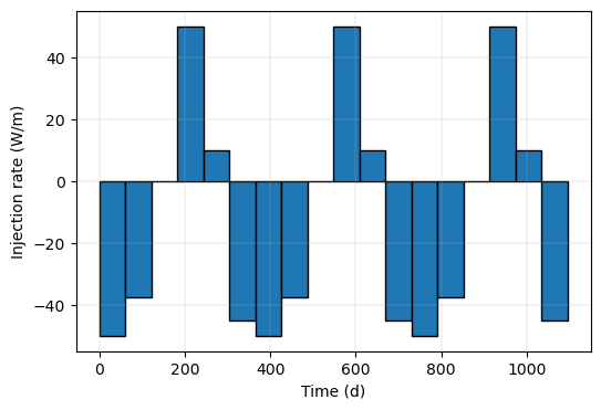
# Time-varying energy loads (W/m) (loosely based on the energy demands in Al-Khoury et al, 2021, fig. 8)
# equal loads for each BHE
# repeat for three years
loads = -np.vstack(
[
np.repeat(50, len(xc)), # january-february
np.repeat(37.5, len(xc)), # march-april
np.repeat(0.0, len(xc)), # may-june
np.repeat(-50.0, len(xc)), # july-august
np.repeat(-10.0, len(xc)), # september-october
np.repeat(45, len(xc)), # november-december
]
)
nphase = loads.shape[0] # number of annual loading phases
nyear = 3
loads = np.vstack([loads] * nyear)
time = (
np.linspace(0, nyear * 365, nyear * nphase + 1) * 86400
) # start time of injection phase, first one should equal 0.0
Finj = np.column_stack([time[:-1], loads]) # used in the analytical solution
# uniform flow using constant-heads
hL = 10.0
hR = hL - (Lx - delr) * grad
chd_pname = "CHD_0" # CHD package name
# stress-period set-up
# The flow simulation has 1 steady-state stress-period
# The energy transport simulation uses 10 time steps for each stress-period
nper = nyear * nphase
nstp = 10
tsmlt = 1.2
tdis_rc = [(t, nstp, tsmlt) for t in np.ediff1d(time)] # using lagged differences
# Solver parameters
inner_dvclose = 1e-6
rcloserecord = [1e-6, "STRICT"]
inner_dvclose_heat = 0.001
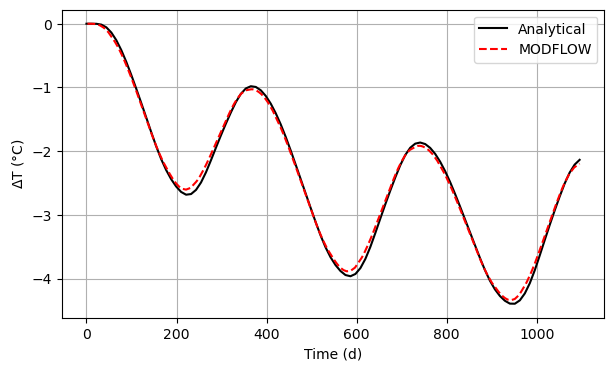
# Arbitrary observation location
obs = (
50 + delr / 2,
40 + delc / 2,
) # x-y coordinates of observation point at cell centroid
obs_time = (
np.linspace(0.0, nyear * 365, 100) * 86400
) # observation times for analytical solution
# Output time and mesh for plotting analytical contours
xg, yg = np.meshgrid(np.linspace(0, Lx, 100), np.linspace(0, Ly, 100))
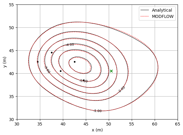
output_kper = 8 # after 1.5 years
[4]:
def build_mf6_flow_model():
    print(f"Building mf6gwf model...{sim_name}")
    sim_ws_flow = sim_ws / "mf6gwf"

    # Instantiate a MODFLOW 6 simulation
    sim = flopy.mf6.MFSimulation(sim_name=sim_name, sim_ws=sim_ws_flow, exe_name="mf6")

    # Instantiate time discretization package
    flopy.mf6.ModflowTdis(
        sim,
        nper=1,  # just one steady state stress period for gwf
        perioddata=[(1.0, 1, 1.0)],
        time_units=time_units,
    )

    # Instantiate Iterative model solution package
    flopy.mf6.ModflowIms(
        sim,
        complexity="SIMPLE",
        inner_dvclose=inner_dvclose,
        rcloserecord=rcloserecord,
    )

    # Instantiate a groundwater flow model
    gwf = flopy.mf6.ModflowGwf(sim, modelname=gwf_name, save_flows=True)

    # Instantiate an structured discretization package
    flopy.mf6.ModflowGwfdis(
        gwf,
        length_units=length_units,
        nlay=nlay,
        nrow=nrow,
        ncol=ncol,
        delr=delr,
        delc=delc,
        top=top,
        botm=botm,
        filename=f"{gwf_name}.dis",
    )

    # Instantiate node-property flow (NPF) package
    flopy.mf6.ModflowGwfnpf(
        gwf,
        save_saturation=True,
        save_specific_discharge=True,
        icelltype=0,
        k=k,
        filename=f"{gwf_name}.npf",
    )

    # Instantiate initial conditions package for the GWF model
    flopy.mf6.ModflowGwfic(gwf, strt=hL, filename=f"{gwf_name}.ic")

    # Instantiating MODFLOW 6 storage package
    # (steady flow conditions, so no actual storage,
    # using to print values in .lst file)
    flopy.mf6.ModflowGwfsto(
        gwf,
        ss=0,
        sy=0,
        steady_state={0: True},
        filename=f"{gwf_name}.sto",
    )

    # Instantiate CHD package for creating a uniform background flow
    chdrec = []
    for j in [0, ncol - 1]:
        if j == 0:
            hchd = hL
        else:
            hchd = hR

        for i in range(nrow):
            chdrec.append([(0, i, j), hchd, T0])

    flopy.mf6.ModflowGwfchd(
        gwf, stress_period_data=chdrec, auxiliary="TEMPERATURE", pname=chd_pname
    )

    # Instantiating MODFLOW 6 output control package (flow model)
    head_filerecord = f"{sim_name}.hds"
    budget_filerecord = f"{sim_name}.cbc"
    flopy.mf6.ModflowGwfoc(
        gwf,
        head_filerecord=head_filerecord,
        budget_filerecord=budget_filerecord,
        saverecord=[("HEAD", "LAST"), ("BUDGET", "LAST")],
    )

    return sim
[5]:
def build_mf6_heat_model():
    print(f"Building mf6gwe model...{sim_name}")
    sim_ws_heat = sim_ws / "mf6gwe"

    sim = flopy.mf6.MFSimulation(sim_name=sim_name, sim_ws=sim_ws_heat, exe_name="mf6")

    # Instantiating MODFLOW 6 groundwater energy transport model
    gwe = flopy.mf6.ModflowGwe(
        sim,
        modelname=gwe_name,
        save_flows=True,
    )

    # Instantiate Iterative model solution package
    flopy.mf6.ModflowIms(
        sim,
        linear_acceleration="bicgstab",
        complexity="SIMPLE",
        inner_dvclose=inner_dvclose_heat,
    )

    # MF6 time discretization differs from corresponding flow simulation
    flopy.mf6.ModflowTdis(sim, nper=nper, perioddata=tdis_rc, time_units=time_units)

    # Instantiate an structured discretization package
    flopy.mf6.ModflowGwedis(
        gwe,
        length_units=length_units,
        nlay=nlay,
        nrow=nrow,
        ncol=ncol,
        delr=delr,
        delc=delc,
        top=top,
        botm=botm,
        filename=f"{gwe_name}.dis",
    )

    # Instantiating MODFLOW 6 heat transport initial temperature
    flopy.mf6.ModflowGweic(gwe, strt=T0, filename=f"{gwe_name}.ic")

    # Instantiating MODFLOW 6 heat transport advection package
    flopy.mf6.ModflowGweadv(gwe, scheme=scheme, filename=f"{gwe_name}.adv")

    # Instantiating MODFLOW 6 heat transport conduction and dispersion package
    flopy.mf6.ModflowGwecnd(
        gwe, alh=al, ath1=ah, ktw=ktw, kts=kts, filename=f"{gwe_name}.cnd"
    )

    # Instantiating MODFLOW 6 energy storage and transport package
    flopy.mf6.ModflowGweest(
        gwe,
        density_water=rhow,
        heat_capacity_water=cpw,
        porosity=n,
        heat_capacity_solid=cps,
        density_solid=rhos,
        filename=f"{gwe_name}.est",
    )

    # Instantiating MODFLOW 6 source/sink mixing package
    sourcerecarray = [(chd_pname, "AUX", "TEMPERATURE")]  # optional when T0 = 0
    flopy.mf6.ModflowGwessm(gwe, sources=sourcerecarray)

    # Instantiating MODFLOW 6 energy source loading package representing the BHE's
    eslrec = {}
    for iper in range(nper):
        eslrec_tr = []
        for i in range(len(xc)):
            cid = gwe.modelgrid.intersect(xc[i], yc[i])
            eslrec_tr.append([(0,) + cid, Finj[iper, i + 1]])
        eslrec[iper] = eslrec_tr

    flopy.mf6.ModflowGweesl(
        gwe,
        stress_period_data=eslrec,
        filename=f"{gwe_name}.esl",
    )

    # Instantiating MODFLOW 6 heat transport output control package
    flopy.mf6.ModflowGweoc(
        gwe,
        budget_filerecord=f"{gwe_name}.cbc",
        temperature_filerecord=f"{gwe_name}.ucn",
        saverecord=[
            ("TEMPERATURE", "ALL"),
            ("BUDGET", "ALL"),
        ],
        printrecord=[("BUDGET", "ALL")],
    )

    # Instantiating MODFLOW 6 Flow-Model Interface package
    pd = [
        ("GWFHEAD", "../mf6gwf/" + sim_name + ".hds", None),
        ("GWFBUDGET", "../mf6gwf/" + sim_name + ".cbc", None),
    ]
    flopy.mf6.ModflowGwefmi(gwe, packagedata=pd)

    return sim
[6]:
def write_mf6_models(sim_gwf, sim_gwe, silent=True):
    # Run the steady-state flow model
    if sim_gwf is not None:
        sim_gwf.write_simulation(silent=silent)

    # Second, run the heat transport model
    if sim_gwe is not None:
        sim_gwe.write_simulation(silent=silent)


@timed
def run_models(sim_gwf, sim_gwe, silent=True):
    # Attempting to run MODFLOW models
    print(f"Running mf6gwf model...{sim_name}")
    success, buff = sim_gwf.run_simulation(silent=silent, report=True)
    if not success:
        print(buff)
    else:
        print(f"Running mf6gwe model...{sim_name}")
        success, buff = sim_gwe.run_simulation(silent=silent, report=True)
    return success


@timed
def run_analytical(sim_gwe, kper, obs, obs_time):
    gwe = sim_gwe.get_model(gwe_name)

    # find corresponding model time of stress-period kper
    temp = gwe.output.temperature()
    kstp = nstp * kper + (nstp - 1)
    t = temp.get_times()[kstp]

    # analytical temperature contours at time kper
    print(f"Running analytical model...{sim_name}")
    cntrs = bhe(
        Finj, xg, yg, t, xc, yc, v, n, rhos, cps, kts, rhow, cpw, ktw, al, ah, T0=T0
    )

    # analytical temperature time series
    ts = bhe(
        Finj,
        obs[0],
        obs[1],
        obs_time,
        xc,
        yc,
        v,
        n,
        rhos,
        cps,
        kts,
        rhow,
        cpw,
        ktw,
        al,
        ah,
        T0=T0,
    )

    return cntrs, ts
Plotting results
Define functions that plot results.
[7]:
def plot_extraction_rates():
    figsize = (6, 4)
    fig, ax = plt.subplots(figsize=figsize)
    ts = np.ediff1d(time)[0]
    t_centered = time[:-1] + ts / 2
    ax.bar(
        t_centered / 86400,
        loads[:, 1],
        width=ts / 86400,
        align="center",
        edgecolor="black",
    )
    ax.set_xlabel("Time (d)")
    ax.set_ylabel("Injection rate (W/m)")
    ax.grid(linewidth=0.2)

    # save figure
    if plot_show:
        plt.show()
    if plot_save:
        fpth = figs_path / f"{sim_name}-injection-rates.png"
        fig.savefig(fpth, dpi=600)

    return
[8]:
def plot_contours(sim_gwe, kper, cntrs):
    gwe = sim_gwe.get_model(gwe_name)

    # get simulated temperature field at end of stress-period kper
    temp = gwe.output.temperature()
    temp_t = temp.get_data(kstpkper=(nstp - 1, output_kper))

    # plot
    lvls = np.arange(-20, 20, 1) + T0
    figsize = (7, 5)
    fig, ax = plt.subplots(figsize=figsize)
    csa = ax.contour(
        xg,
        yg,
        cntrs,
        levels=lvls,
        colors="black",
        linewidths=0.8,
        negative_linestyles="solid",
    )
    pmv = flopy.plot.PlotMapView(gwe, ax=ax)
    cs = pmv.contour_array(
        temp_t,
        levels=lvls,
        colors="red",
        linewidths=0.8,
        negative_linestyles="dashed",
        linestyles="dashed",
    )
    plt.clabel(cs, fmt="%.2f", fontsize=8, colors="black", inline=False)
    ax.set_xlabel("x (m)")
    ax.set_ylabel("y (m)")
    ax.scatter(obs[0], obs[1], marker="x", color="green")
    ax.scatter(xc, yc, marker=".", color="black")
    ax.set_axisbelow(True)
    ax.grid()
    ax.set_aspect("equal")
    ax.set_xlim(30, 65)
    ax.set_ylim(30, 55)
    h1, _ = csa.legend_elements()
    h2, _ = cs.legend_elements()
    ax.legend([h1[0], h2[0]], ["Analytical", "MODFLOW"])

    # save figure
    if plot_show:
        plt.show()
    if plot_save:
        fpth = figs_path / f"{sim_name}-contours.png"
        fig.savefig(fpth, dpi=600)

    return
[9]:
def plot_ts(sim_gwe, obs, ts):
    gwe = sim_gwe.get_model(gwe_name)

    # get simulated temperature series at location
    obs_ij = gwe.modelgrid.intersect(obs[0], obs[1])
    temp = gwe.output.temperature()
    obs_temp = temp.get_ts((0,) + obs_ij)

    # plot
    figsize = (7, 4)
    fig, ax = plt.subplots(figsize=figsize)
    ax.plot(obs_time / 86400, ts, label="Analytical", color="black")
    ax.plot(
        obs_temp[:, 0] / 86400,
        obs_temp[:, 1],
        label="MODFLOW",
        color="red",
        linestyle="dashed",
    )
    ax.set_xlabel("Time (d)")
    ax.set_ylabel(r"$\Delta$T (°C)")
    ax.grid()
    ax.legend()

    # save figure
    if plot_show:
        plt.show()
    if plot_save:
        fpth = figs_path / f"{sim_name}-ts.png"
        fig.savefig(fpth, dpi=600)
[10]:
def scenario(idx, silent=False):
    sim_gwf = build_mf6_flow_model()
    sim_gwe = build_mf6_heat_model()

    if write and (sim_gwf is not None and sim_gwe is not None):
        write_mf6_models(sim_gwf, sim_gwe, silent=silent)

    if run:
        success = run_models(sim_gwf, sim_gwe, silent=silent)
        if success:
            cntrs, ts = run_analytical(sim_gwe, output_kper, obs, obs_time)

    if plot and success:
        plot_extraction_rates()
        plot_contours(sim_gwe, output_kper, cntrs)
        plot_ts(sim_gwe, obs, ts)
[11]:
scenario(0, silent=True)
Building mf6gwf model...ex-gwe-bhe
Building mf6gwe model...ex-gwe-bhe
Running mf6gwf model...ex-gwe-bhe
Running mf6gwe model...ex-gwe-bhe
run_models took 4781.52 ms
Running analytical model...ex-gwe-bhe
run_analytical took 6818.88 ms